Optimal certainty-equivalent spending retirements with DataNitro
*Let’s see if we can come up with an ideal spending plan for a retirement, if you have a guaranteed annual return, for different levels of risk aversion. * It’s probably been done before, but seems like a fun illustration of the power of numerical optimization with Excel, Python and DataNitro.
A toy problem.
Suppose you are a 111-year-old male, and you would like to know how much to spend the rest of your retirement.
You look up a life table _ you see it gives you 100% probability of dying this year (rounded _ 1 life out of 10,000 survives to 111, 0 to 112)
How much of your portfolio should you spend this year to maximize your lifetime spending?
The answer is obvious — 100%! There is no risk of shortfall in future years, assuming this life table holds up.
Now let’s suppose you are 110. According to the life table, 2 lives out of 10,000 survive to 110. One shuffles off this mortal coil at 110, the other at 111.
Suppose you have a guaranteed 5% real return. How much should you spend each year to maximize lifetime spending?
If you save $1, you can spend $1.05 if you’re still alive to spend it. But you have only a 50% chance of being alive. So every dollar you save is worth $0.525 in lifetime spending. Every dollar you spend now is worth $1.
So once again, you should spend the entire portfolio!
More generally, as long as the future value is higher than the 1/probability of being alive, you save the entire amount. As soon as the future value is less than 1/probability of being alive, you spend everything.
You spend everything if:
Otherwise you spend nothing. To maximize lifetime income, you spend nothing until you reach maximum bang for the buck, so to speak, then you spend the entire portfolio.
Of course, in the real world, this is not a recommended or preferred retirement plan.
The CRRA utility function
Real people care about the variability and risk of their income stream. To quantify that, we can use a constant relative risk aversion (CRRA) utility function.
The intuition behind a CRRA utility function is that given a choice between
1) flipping a coin to get either $10 or $15, and
2) a certain $12.50,
the risk-averse retiree prefers a certain payoff to a risky payoff with the same expected value.
The form of a CRRA function is:
![]()
Where U is utility, C is consumption (spending), and γ (gamma) is the risk-aversion coefficient.
A highly risk-averse person (high γ) might value the risky payoff at $11, the certainty-equivalent (CE) value of the coin-flip. A less risk-averse person might want at least $12 (γ =2), and only a risk-neutral person would accept $12.50. No rational person accepts a certain $10 v. a minimum $10 and a chance at $15.
Constant relative risk aversion refers to the property that the size of the bet doesn’t matter – if the certainty-equivalent value of a $100/$150 coin-flip is $120, then the CE value of a $1000/$1500 coin-flip is $1200.
The table below shows certainty equivalent values of a $10/$15, and $100/$150 coin flips for different levels of γ.
| CE(10,15, γ =8) | $10.95 |
| CE(10,15, γ =4) | $11.56 |
| CE(10,15, γ =2) | $12.00 |
| CE(10,15, γ =1) | $12.247 |
| CE(10,15, γ =0) | $12.50 |
| CE(100,150, γ =8) | $109.52 |
| CE(100,150, γ =4) | $115.55 |
| CE(100,150, γ =2) | $120.00 |
| CE(100,150, γ =1) | $122.47 |
| CE(100,150, γ =0) | $125.00 |
We can similarly discount an uneven stream of cash flows, ie $15 followed by $10, using the same CRRA utility function. It’s just a consistent way of discounting the variability of the income stream, either over time or a probability distribution.
So now, let’s evaluate that 110-year-old’s retirement for different levels of gamma. Let’s find the spending that maximizes the CRRA utility function for different levels of gamma.
| γ | Age 110 | Age 111 |
| γ = 0 | 100% | 0% |
| γ = 1 | 71.9% | 100% |
| γ = 2 | 62.7% | 100% |
| γ = 4 | 59.1% | 100% |
| γ = 8 | 57.2% | 100% |
We can go back further, to age 109, 108, 65, even back to age 1. Then we can plot what spending would look like for someone who starts off with a $1m portfolio at birth.
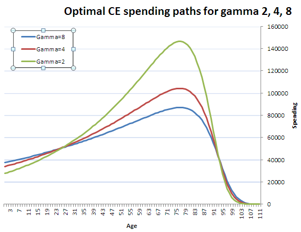
Voilà! Given a guaranteed 5% real return, and a risk aversion coefficient γ, these are the the spending paths that would have maximized CRRA utility, or certainty-equivalent spending.
Someone who retires at age 65, or any age, could pick the curve that matches their risk aversion, and just use the part of the curve starting at that age, prorating spending to match the size of their initial portfolio.
The intuition of the drop off after age 80 is, to get income at say 95, when your odds of being alive are low, you have to give up a lot of income at say 70. So if you want to maximize lifetime income, buying life insurance, joining an insurance pool and annuitizing those later years makes more sense saving for them all by yourself. Effectively, life insurance is like five people who each need $1 for the year where 20% of them are alive, so each only has to put in $0.20, and the one who lives gets the whole amount.
Hmmh… I wonder if it’s possible to run this same optimization without the 5% real return assumptions, but over historical stock and bond returns instead… To be continued.