Asset Allocation for Midwits: Everything You Always Wanted to Know About Portfolio Optimization But Were Afraid to Ask

You don’t need to be a rocket scientist. Investing is not a game where the guy with the 160 IQ beats the guy with 130 IQ. Success in investing doesn’t correlate with IQ once you’re above the level of 120. What you need is the temperament to control the urges that get other people into trouble in investing. If your IQ is 150, sell 30 points; it won’t hurt. - Warren Buffett

Efficient Frontier using US Asset classes, 1928-2025

Today we will revisit portfolio theory, which I have posted about in the past, and try to present a coherent introduction to portfolio optimization and asset allocation, with data through 2025 and vibe-coded illustrations.

I would like to explain some things that were not explicitly made clear to me when I first encountered portfolio theory, and build a reasonably robust long term allocation from data and first principles.

The capital asset pricing model was popularized by Harry Markowitz and William Sharpe, although several people came up with versions of it independently. It lets you identify optimal risk/reward portfolios, if you make some (not 100% realistic) assumptions about how asset prices behave.

Ultimately we want to get to a useful version of the charts below.

This efficient frontier chart shows feasible combinations of risk and reward.

This transition map shows the composition of efficient portfolios at different levels of risk. Mouse over to see historical returns and asset composition:

We’ll proceed as follows:

1. Why volatility is a proxy for risk.
2. Why volatility is an imperfect proxy for risk.
3. Visualizing volatility math with pictures of triangles.
4. Visualizing optimal portfolios with efficient frontiers.
5. Picking an optimal portfolio.
6. Regularization and backoff - the midwit way.
7. Various scientific alternatives.
8. Conclusion: the data is sparse and ill-behaved, the math is not super realistic, but this gives us a reasonable starting point.

I hope you’ll have a better understanding of how to make reasonable decisions about allocations based on past market behavior and a little math.

Disclaimer: this is educational material, not financial advice.

1. Why volatility?

Suppose you are watching a peaceful ocean, and suddenly a shark eats a lone swimmer. That’s a bad outcome. The risk was probably there all along, but we didn’t perceive the risk because we weren’t aware of the possibility of a very bad outcome.

On the other hand, if you are watching Jaws, and you see the shark’s fin gliding toward unsuspecting swimmers, bad stuff could happen. Either the lifeguard will blow his whistle and they will narrowly escape being attacked, or someone will meet a grisly fate. We sense the danger. Suspense mounts, and our pulse quickens.

Risk means the future can follow many paths, including good and bad ones, but only one path will happen.

We can represent this as a probability distribution of possible outcomes. Less risky portfolios have narrow distributions clustered around the mean, with some better and some worse outcomes. Riskier portfolios have a wider confidence interval, with some extremely bad and some extremely good outcomes.

What this looks like in the market is this:

Notably, percentage return calculations are asymmetric in the sense that a 50% rise from 100 to 150, followed by a 50% drop to 75, leaves you down 25%. A 10% rise is the same number of dollars as a 10% drop, but it’s harder to catch up from the loss since your base is now smaller. The log diff of the total return index, i.e. \(log(1+r)\) where \(r\) is the percent return, is a more symmetric representation of change, and this chart of log diff returns is more representative of the fat tails (leptokurtosis) and left skew in returns, with most returns to the right of the mean and fat tails on the left.

Why is volatility used to measure risk? Volatility is the standard deviation of returns, and measures the size of typical daily (or longer, or shorter) swings. Volatility measures the width of the bell curve, or the range of possible outcomes. Historical volatility measures the size of past swings. Implied volatility measures what options price in about future swings. Lower volatility means outcomes are fairly predictable; higher volatility means a lot of different outcomes are possible.

Consider Ben Graham’s metaphor of manic-depressive Mr. Market.

One of your partners, named Mr. Market, is very obliging indeed. Every day he tells you what he thinks your interest is worth and furthermore offers either to buy you out or to sell you an additional interest on that basis. Sometimes his idea of value appears plausible and justified by business developments and prospects as you know them. Often, on the other hand, Mr. Market lets his enthusiasm or his fears run away with him, and the value he proposes seems to you a little short of silly.

On a typical day, bipolar Mr. Market swings a typical amount between euphoria and despair.

That volatility tells you how risky Mr. Market thinks the stock is, as a first-order approximation. In the short run, volatility just tells you market perception of risk. In the long run, it incorporates the good and bad things that actually did happen, and more closely approximates true risk.

Even then, a lot of things that could have happened didn’t happen. Maybe there was a too-great or not-great-enough probability of a disastrous war priced into the swings during the Cuban Missile Crisis. The concept of ‘risk’ is a Platonic ideal of things that are not knowable and don’t necessarily follow distributions you can model. Any attempt to put a number on it is inherently subjective. Still, volatility measures the range of returns that investors actually experienced, and what risk the market prices in, and these are good to know.

We usually express volatility at an annual rate. We can do that because if you assume well-behaved log-normally distributed returns, then there is a simple relationship between daily volatility, monthly volatility, and annual volatility.¹

Let’s look at the distribution of stock returns over longer time frames.

We see tighter distributions as we look at longer spans. Many of the 20-year time spans overlap, so this probably overstates the convergence. But note that there has never been a 20-year negative real return in the S&P. If returns are uncorrelated and well behaved, we should expect returns over longer periods to converge toward the mean return according to a square root law. You are not guaranteed a great return, but if you stay invested for a long time the law of averages is on your side.

Let’s look at the distribution of real returns of various assets:

We can see that assets with high volatility tend to have higher mean returns:

	Mean Return	Geometric	STD
GDP	0.033020	0.031945	0.047254
CPI	0.031108	0.030374	0.039154
S&P	0.085485	0.067000	0.193954
Small Caps	0.141127	0.084081	0.372102
T-Bills	0.003392	0.002675	0.038017
T-Notes	0.018030	0.014209	0.088987
Baa Corps	0.038531	0.034818	0.088440
Real Estate	0.012791	0.011557	0.049934
Gold	0.034768	0.020178	0.186131

The more risky an asset is, the higher the return investors demand to hold it. (Gold is an outlier; its negative correlation with the other assets, and reputation for holding its real value over the long run in spite of inflation make people hold it, in spite of high volatility.)

More to the point, investors really care about nondiversifiable risk. Truly random, idiosyncratic volatility in a financial instrument is not a big deal if you can buy 20 securities with that type of risk which cancel each other out.

Why are some assets more volatile than others? Fixed income assets have a fixed payout, but longer duration can make them more sensitive to variations in interest rates. Some companies have higher variability in earnings, or may have no earnings and be a crapshoot, like a speculative drug or tech company. The earnings are farther in the future and duration comes into play. Also, if a company has a lot of debt and fixed expenses, i.e. high financial and operating leverage, then a swing in expectations about business conditions might impact future earnings and the stock price a lot more than an unlevered stock with very consistent earnings.

2. Issues with volatility

A model of log normal distributions is not totally realistic in practice:

• As seen above, we have asymmetric fat tails (the volatility smile). Why? Extreme events happen more frequently than predicted by normal distributions. Extreme negative events happen more frequently than equally extreme positive events. We have meltdowns but not meltups. We have seen nuclear power plants melt down into a pile of rubble and melted fuel. We have never seen a pile of rubble melt up into a working nuclear power plant. Entropy says you can demolish a building almost instantaneously with well-placed explosives, but you can’t construct a building the same way, however well you place the explosives.

• We have serial correlation. Markets can trend. Information can take time to be fully understood and reflected in stock prices. A decision a board or investment committee makes one day might result in many changes to companies or portfolios over long periods. Investor psychology is durably impacted by the recent past. Investors can also overreact and mean-revert. A high Shiller PE is associated with lower future returns. And people have loss aversion and a healthy fear of entropy and not being able to buy a GI Joe with a Kung Fu grip, and suffer from herding and crowd psychology. They will rush to sell when it’s down 40% and then rush to buy when it’s up 40%. Trending and mean-reversion can coexist at different time scales and for different types of perturbations.

• We do not have covariance stationarity. The S&P today, with >40% in Big Tech, has different risk/return characteristics compared to say 1980 energy-heavy stocks or 1960 manufacturing stocks. We have regime changes based on changes in economic and market structures like the gold standard, international trade, monetary and fiscal policy regimes. Observed volatility measures what Mr. Market thinks at a given time. Mr. Market evolves over time and what Mr. Market thinks today might not be an accurate reflection of the future. Past performance does not predict future results.

• Nonlinearity. Companies have complex dynamics that are not fully described by linear relationships over longer time periods and larger changes in the environment. Consider two identical companies, like gold mines, whose earnings depend on the price of gold and the cost of mining it. Suppose one decides to lever up and distribute cash. If the gold price goes down a lot, the unlevered company may no longer be profitable but it still owns the gold mine and the possibility of being profitable in the future. The second, levered company is bankrupt. The debtholders take over the mine to recover the debt, and the stock is worthless. On the other hand, if the stock goes up a lot, the second company organically delevers and the economics become similar to the first company. There is positive convexity, investors keep the upside and bondholders get a lot of downside in exchange for interest payments. At a high price the stocks may have a beta of 1 and a high correlation. At lower prices the levered one has a higher beta. Correlation is a first-order measure of how things move together, it doesn’t accurately reflect higher-order derivatives and the dynamics of large price moves.

• Investors may have complex distributional preferences that aren’t well described by volatility. For instance, they might care mostly about downside volatility in an asymmetric loss averse psychological model, maybe like Kahneman-Tversky prospect theory. Humans can be weird and boundedly rational. But weird utility functions make the math intractable, and lead to path dependencies and time inconsistencies. It’s hard to reason about unreasonable things.²

Humans don’t have a linear utility relationship with volatility. Markets don’t exhibit log normal behavior in realized returns. As Einstein said, if you want to describe reality correctly, you must leave elegance to the tailor. Some degree of mathematical perversity is a feature of real human beings and real financial markets.

Nevertheless, it is useful to start from tractable assumptions and simple models we can reason about, and see what they tell us. Even if they are imperfect in practice, they teach us useful ways to think. And from there maybe we can relax assumptions and build more realistic models.

Keeping these imperfections in mind, let’s proceed, with an awareness of monsters lurking below the surface.

3. Visualizing volatility math with triangles

The relationship between the volatility of individual stocks and the volatility of a portfolio of stocks can be expressed using the volatilities and correlation of returns, and visualized with vector addition.

Interactive visualization of portfolio risk using vector addition
Drag the slider to set the correlation between the 2 assets.

Correlation (ρ)

-1.000 0.000 +1.000

Recall that the correlation is the change in expected return of one stock conditioned on the change in expected return of the other, each expressed in units of the number of standard deviations.

Suppose we have 2 stocks with actual returns \(r_1\) and \(r_2\), expected (mean) returns \(\mu_1\) and \(\mu_2\), standard deviations \(\sigma_1\) and \(\sigma_2\) and correlation \(\rho_{12}\). Then:

\[\frac{\hat{r}_2 - \mu_2}{\sigma_2} = \frac{\hat{r}_1-\mu_1}{\sigma_1} \rho_{12}\]

If the realized return \(r_1\) of stock 1 is 1 SD higher than its expected value \(\mu_1\), then the expected return of stock 2 \(r_2\) is \(\rho_{12}\) SDs higher than its expected value \(\mu_2\).

Correlation	Return of stock \(1\)	Expected return of stock \(2\), given return of stock \(1\)
\(\rho_{12}=1\)	\(\mu_1 + \sigma_1\)	\(\mu_2 + \sigma_2\)
\(\rho_{12}=0.5\)	\(\mu_1 + \sigma_1\)	\(\mu_2 + 0.5\sigma_2\)
\(\rho_{xy}=0\)	\(\mu_1 + \sigma_1\)	\(\mu_2\)
\(\rho_{12}=-1.0\)	\(\mu_1 + \sigma_1\)	\(\mu_2 -\sigma_2\)

If we have a portfolio of these 2 stocks, the return of the portfolio is the weighted average of the two returns: \(r_p = w_1r_1 +w_2r_2\) where \(w_i\) is the weight of stock \(i\) between 0 and 1 and \(r_i\) is the return of stock \(i\).

The volatility of this portfolio is given by

\[\sigma_{p} = \sqrt{(w_1\sigma_1)^2 + (w_2\sigma_2)^2+ 2w_1\sigma_1 w_2\sigma_2\rho_{12}}\]

This is a vector addition. Suppose we have a triangle of 3 vectors \(\vec{a}\), \(\vec{b}\), and \(\vec{c}=\vec{a}+\vec{b}\), and an angle \(\theta\) between \(\vec{a}\) and \(\vec{b}\). Denote the length of the three sides as \(a\), \(b\), \(c\) (properly \(\lVert \vec{a} \rVert ,\lVert \vec{b} \rVert ,\lVert \vec{c} \rVert\)).

Then the length of the 3rd side \(c\) is given by:

\[c = \sqrt{a^2 + b^2+ 2a b\cos \theta }\]

The equation for \(c\) has a form analogous to the equation for \(\sigma_{p}\), with correlation standing in for cosine.

If we define \(a=w_1\sigma_1\), \(b=w_2\sigma_2\), then we can draw a triangle with 2 sides of length \(a\) and \(b\). We set the angle \(\theta\) so \(\cos \theta\) = \(\rho_{12}\). Then the length \(c\) of the third side of the triangle represents the volatility of the portfolio of the 2 stocks.

The rest of this is strictly optional but if you define the portfolio weight vector:

\[\mathbf{w} = \begin{pmatrix} w_1 \\ w_2 \end{pmatrix}\]

and the correlation matrix of these 2 stocks:

\[\mathbf{R} = \begin{pmatrix} 1 & \rho_{12} \\ \rho_{12} & 1 \end{pmatrix}\]

and a diagonal matrix to scale it by the standard deviations:

\[\mathbf{D} = \begin{pmatrix} \sigma_1 & 0 \\ 0 & \sigma_2 \end{pmatrix}\]

then the covariance matrix is

\[\Sigma = \mathbf{D} \mathbf{R} \mathbf{D} = \begin{pmatrix} \sigma_1^2 & \rho_{12}\sigma_1\sigma_2 \\ \rho_{12}\sigma_1\sigma_2 & \sigma_2^2 \end{pmatrix}\]

And you can write the formula for the portfolio variance as:

\[\sigma_p^2 = \mathbf{w}^\top \Sigma \mathbf{w}\]

And that formula generalizes to \(n\) assets with an \(n \times n\) covariance matrix \(\Sigma\) and a weight vector of \(n\) asset weights. A useful bit of notation, since large portfolios have a lot of terms.

This formula is an identity. It does not depend on returns being log-normally distributed. However, if returns are log-normally distributed, then so is the portfolio return. A 68–95–99.7 rule will hold. If you have deviations from normality, the formula will still hold, but the interpretation may be very different.

4. Visualizing optimal portfolios with efficient frontiers

Let’s build an efficient frontier which is a great way to visualize the risk and return of feasible portfolios.

We use data on major asset classes from Aswath Damodaran.

Descriptions of the data are in the 1st tab of the histretSP.xls Excel spreadsheet.

Stocks (Large Cap)	S&P 500
Stocks (Small Cap)	Ken French bottom decile
US T.Bill	Average 3-month Treasury bill rate
US T.Bond	10-year Treasury bond constant maturity return
Aaa & Baa Corporate Bond	Moody’s Aaa and Baa returns
Real Estate	Case-Shiller Index (residential, price only)
Gold	Gold price per oz.

We can compute an efficient frontier, showing the best feasible combinations of risk (vol) and return, using the following process:

1. Estimate the covariance matrix of all the assets.
2. Find the maximum return portfolio, which is 100% of the highest mean return asset.
3. Find the minimum volatility portfolio via gradient descent (convex optimization).
4. Split the space between the max return vol and min vol into e.g. 200 equally spaced points.
5. For each vol \(\sigma_i\), find the portfolio weights that maximize the weighted average return, subject to a constraint of at most that vol, \(\sigma_p < \sigma_i\).
6. Plot the resulting portfolio returns vs. the portfolio vol.

Minimizing volatility (or maximizing return) is a convex optimization problem. ‘Convex’ means the return surface in weight space is like a big hill with a single peak, with no local maxima or saddle points. So if we just always move in the direction that gives better results, we are guaranteed to reach the best solution.

In math terms, we can solve a convex optimization problem by gradient descent. By convention we optimize in the direction of a minimum like the negative of the return. If the 2nd derivatives (Hessian in multiple dimensions) are nonnegative everywhere, then if we keep going downhill, then the first local minimum we find, where any weight change in any direction moves volatility up, is also the global minimum. Also, if you add constraints like “weights must sum to 1”, which form a boundary around the search space, the feasible space defined by constraints must be convex and not some weird shape, where gradient descent could lead you to a corner solution at a binding constraint, even if starting from somewhere else would lead you to a different, better solution.

We can use cvxpy which is a framework by Stephen P. Boyd that lets you use various optimization problem solvers.

We get this efficient frontier, the blue line, which shows the maximum mean return you can get for any portfolio risk budget.

Why the orange line? After computing the blue line, which is the portfolio’s mean return over the time span, I wanted to calculate the annualized percentage return, i.e. the geometric mean, for each optimal portfolio on the efficient frontier. I wanted to check the math that came out of the optimization. To compute the orange line, I took the asset weights for each portfolio on the blue line, and simulated its actual performance, rebalancing annually, and calculated its realized vol and realized annualized return. The math checked out, the blue line shows the optimal mean returns. But remember when we said percentage changes are asymmetric? When we simulate the portfolio, the geometric mean return is lower than the arithmetic mean return, because of volatility drag. The more volatile assets go up and down a lot, and if they go up 10% to 1.1 and down 10% to 0.99, the arithmetic mean return is 0, but the geometric return is down 1%.

Fortunately there is a trick we can use to improve our optimization. The geometric return including volatility drag can be estimated by average return - variance/2 . In our optimization, if we maximize this adjusted return of \(\mu -\sigma^2 / 2\), we get these efficient frontiers:

Maximizing the return less estimated volatility drag is very close to the actual realized efficient frontier using the estimated optimal portfolios.

Note: the efficient frontier stops before the ‘small cap’ marker, because it turns out that is not an efficient portfolio. Adding a bit of S&P to a 100% small cap portfolio reduces volatility, since S&P is less volatile, and also actually increases return, by reducing volatility drag.

Finally we can visualize individual portfolios via this transition map which shows how the portfolio evolves as you tolerate higher and higher risk (roll over for asset weights).

5. Picking the optimal portfolio on the frontier

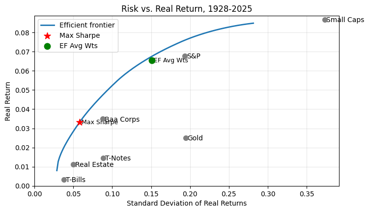
There is a smart way to pick a good portfolio, which chooses the red star, and a midwit way, which chooses the green star.

First, the genius way:

• Let’s assume there is a risk-free rate on cash of 0%, which you can achieve with a volatility of 0%. Since we are using real returns, this means something that yields exactly the CPI every year. A guaranteed pre-tax return of CPI + some coupon is achievable with TIPS. The vol will only be 0 in real terms if you e.g. donate the coupons.
• If you add this risk-free asset to the mix, it is a marker at the origin.
• Then you can combine this risk-free asset with any portfolio on the efficient frontier and your return will be a weighted average of the risk-free rate of 0% and the chosen portfolio return.
• If you draw a line from (0, 0) so it is tangent to the outermost point of the efficient frontier, then the tangent portfolio is the portfolio with the maximum Sharpe ratio, which is defined as \((r_{portfolio} - r_{riskfree} ) / \sigma_{portfolio}\). It’s how much return you pick up over the risk-free return per unit of risk. You can combine the Sharpe-optimal portfolio with some amount of cash to achieve any risk-return profile on the dotted line.
• Then suppose you can borrow at some rate less than the return on your portfolio. For simplicity’s sake assume it’s the same 0% real rate. Then if you continue the line to the right of the Sharpe-optimal portfolio, that represents borrowing at 0% and buying more of the Sharpe-optimal portfolio. If you can borrow at e.g. 2% then the line will be a little flatter and be tangent to the efficient frontier starting a bit further right where the slopes line up.

Every point on this capital market line is a feasible portfolio with the same Sharpe ratio. In Sharpe world, you should always buy the risk asset portfolio with maximum Sharpe ratio. And then lever it up for more risk and return, like a hedge fund, or lever it down combining it with the risk-free asset if you prefer lower risk and return.

But there are some problems with this in our world:

1. We are trying to maximize real returns after inflation. On the one hand, there isn’t actually an asset that pays the CPI flat. On the other hand, TIPS should do better, but with some modest volatility. Ideally we would add TIPS to the asset universe. But they’ve only been around the last 30 years or less. We could try to model what TIPS returns would have been historically by estimating historical inflation expectations based on current inflation, the monetary/fiscal policy mix, other predictors like yield curves, gold prices, FX etc., and add some noise to match correlations. But that’s a rabbit hole. Assuming a zero return asset isn’t accurate, but it’s not crazy, it’s a little less return and volatility than is actually achievable.

2. Most retail investors can’t or don’t use leverage. You can invest on margin, but the margin rate is high. If you borrow, there is a path dependency where you get liquidated if your equity gets too low or negative. If the borrowing rate varies, that would have to be reflected in the optimization. Retail investors typically want to move to the right to increase their risk and return, and not simply lever up.

3. There is the complex problem of overfitting. We have taken average returns of assets and covariances over a long period. But we don’t really know how accurate these are as a forecast over our time horizon. And optimal portfolios are highly sensitive to return and covariance forecasts. In fact, optimization tends to maximize estimation errors. The better your optimal portfolio, the more likely it takes advantage of unlikely quirks in the forecasts.

In machine learning, we generally regularize to avoid overfitting. if we perform a regression, we typically add a penalty to parameters to shrink them toward 0, and the estimator toward the mean. We use cross-validation to determine how much to regularize, and balance overfitting and underfitting, by checking what regularization parameters generalize best out-of-sample.

This can be viewed as a Bayesian approach, where we start with a maximum entropy prior. For instance: a naive base case might be that all parameters are 0 with some distribution; then we update the prior in proportion to the strength of the evidence they are greater than 0. L2 regularization implies a Gaussian prior on parameter distribution, L1 implies a Laplacian prior.

Knuth has been quoted as saying, the root of all evil is premature optimization. Which is exactly the same as overfitting to an imperfect understanding of the problem. Bad government policy = overfitting to past problems. Bad heuristics and prejudices = overfitting to personal experience or what your grandparents or your lizard brain taught you. It takes a lot of wisdom to only learn from data in proportion to the evidence. You have to have a good model for how the evidence was created and what the underlying reality might look like.

Frequentists may object to a Bayesian approach because it seems non-mathy, where does this prior belief come from? On the other hand, even if you don’t use an implicit prior in linear regression, you can back a prior out via Bayes’s law, like a continuous distribution from -infinity to +infinity. So I would argue everyone is a Bayesian, but non-Bayesians don’t make priors explicit. The real question is whether a Bayesian prior improves out-of-sample performance, and it often does. If you use a prior distribution on IMDB movie ratings, you get a better rating sooner with fewer incoming votes. If you have some information about what the model should look like, you should use it, otherwise you are not getting the best model. Of course, you should only use the most defensible maximum-entropy prior, otherwise you might be introducing bias into your model.

If we don’t systematically regularize, our model will overfit and not generalize well out of sample.

As far as I know, there is no generally accepted way to do this for portfolio optimization. So, here is a midwit way to back off the optimized portfolio toward one that is more robust to estimation errors: just average all the optimal portfolios.

That gets us the green star, which looks like this:

Average over entire efficient frontier:

Real Return	6.56%
SD	15.09%
Sharpe Ratio	0.434

Asset	Weight
S&P	34.3%
Small Caps	23.1%
T-Bills	3.1%
Baa Corps	15.9%
Real Estate	8.5%
Gold	15.1%

This is admittedly a very simplistic, possibly stupid methodology that loses Sharpe ratio, but not very much. The portfolios at the extremes are probably not ones you would realistically choose. You might want to average over the reasonable portfolios in the middle. But we could view it as a base case.

If we add a risk-free asset we get this.

Average over entire efficient frontier:

Real Return	6.06%
SD	13.73%
Sharpe Ratio	0.442

Asset	Weight
S&P	31.3%
Small Caps	20.8%
Baa Corps	15.7%
TIPS	11.1%
Real Estate	7.1%
Gold	13.9%

A risk-free asset unsurprisingly can help reduce your risk.

In general, inflation is a risk you want to protect against in a portfolio. It was a big deal in the 70s. The current policy mix may tend toward the inflationary: large fiscal deficits, political pressure on the Fed, tariffs, deglobalization, dollar depreciation, and labor market tightness exacerbated by immigration crackdowns.

Stocks offer some inflation protection over the long run. Buffett would probably argue against gold and TIPS generally, because they are low or zero-yielding assets, and a bet against the rationality and wisdom of policymakers. Also, if you are Buffett, your opportunity set is a bit different, if you can reliably find equities that will give you inflation protection in the form of moats and brand equity and pricing power over the very long haul, plus equity risk premium. Inflation protection is expensive if it means giving up equity risk premium. The index investor disclaims any such ability and is more at risk. In any event, these portfolios should be considered a starting point for thinking, not a substitute for it.

TIPS offer an inflation hedge and a safe real return, so they might dominate gold. In my opinion, there isn’t a strong theoretical argument gold should increase in value faster than inflation in the long run (gold bugs might disagree and think fiat currencies go to zero, but that’s my story and I’m sticking to it). I could see reasonable arguments why gold should maintain its real value: As the world gets richer, people may want the same value of jewelry in proportion to their wealth, the supply of gold is fairly fixed, with mining and industrial consumption resulting in little net change, and thus gold prices may keep pace with other assets. Also, there is monetary demand for gold; when people lose confidence in monetary authorities and fiat currency holding value, they demand gold because it is currency-like and supply is relatively fixed. So gold offers an inflation hedge.

The real estate series we have is the Case-Shiller index. Real estate is an important asset class, but this index is not investable. Some investors may have homes and already be exposed to real estate. Others would probably prefer liquid real estate ETFs, but we don’t have data on them until recently. If we take out real estate, the analysis looks like this:

Average over entire efficient frontier:

Real Return	6.03%
SD	13.73%
Sharpe Ratio	0.439

Asset	Weight
S&P	31.5%
Small Caps	20.8%
Baa Corps	16.8%
TIPS	17.1%
Gold	13.8%

6. More scientific ways to pick an optimal portfolio

There is no generally accepted way to regularize this analysis, but there is a lot of work in this area, here are a few approaches:

• Ledoit-Wolf covariance matrix shrinkage - More robust covariances that work better out of sample.

• Just add a vol penalty to the optimization to force a lower risk, more diversified portfolio at each level of return. We are already adding a vol penalty to adjust for volatility drag. We can increase the penalty, and my theory is, this will force a more diversified portfolio and be more robust to estimation error. This begs the question of how big a penalty. We could do leave-one-out cross-validation or a similar Monte Carlo process to compute a Sharpe-optimal portfolio on many penalty parameters, and plot the average return, SD and Sharpe ratio for held-out data vs the penalty parameter, to find what works best out of sample. The machine learning engineer in me says go for it, the midwit finance/statistics guy finds it hard to justify rigorously. Left as an exercise.

• Near optimal portfolios One approach is, first find the highest Sharpe portfolio. Then we can say, find the lowest risk portfolio with no more than e.g. a 0.05 drop in Sharpe ratio. Since this portfolio is more diversified, i.e. most diversified within 0.05 of maximum Sharpe, it should be more robust out-of-sample.

• Subset resampled portfolios, Suppose we have 6 assets, do 6 optimizations, dropping one asset each time, then average all the portfolios. Similar to random forest, an ensemble of intentionally weakened models can perform better out of sample than a single overfitted model.

• Michaud resampling and MCOS. Do Monte Carlo simulations where we perturb the return forecasts and covariances randomly each time, and average all the resulting portfolios.

• Hierarchical Risk Parity and related methods like Nested Cluster Optimization. Create a tree of assets clustered by similarity. Then starting at the bottom at each non-leaf create a risk parity portfolio of assets under the node, and recursively climb the tree to get a global portfolio. If you create a portfolio of t-bonds and notes and bills and corporates (NCO) and MBS and munis, we will get some of each, even if one is dominated under MV optimization. Same if you do US stocks and various international markets with different market caps and geographies. Then as you combine clusters, all asset classes are represented, whereas a global optimization might omit some assets. Vanilla HRP actually ignores returns and substitutes cluster hierarchy for the covariance matrix, and creates a minimum risk portfolio assuming no covariance at each level. Which ignores a lot of information. Schur portfolios let you split the difference between vanilla HRP and optimization using the return and covariance information.

If you can come up with a good set of assumptions and a reasonable way to regularize covariance matrices and return forecasts and generate optimal portfolios that generalize well out of sample, you can gain fame and fortune.

7. Concluding thoughts

What have we learned?

• Markets are complex. All models are wrong (George Box), but some are useful. We didn’t even go into issues with the single-index beta model.
• Visualizing portfolio composition as vectors and correlations as cosines can help build intuition about volatility, correlation and diversification.
• The importance of regularization. You probably don’t have very good forecasts, and even really smart and sophisticated investors get burned by leverage. For instance before the financial crisis, Citibank and Harvard both decided they should be taking more risk and leverage and got burned. Famously, the geniuses at Long Term Capital Management made highly levered bets on relatively sure things like buying illiquid off-the-run bonds and selling liquid on-the-run bonds, only to lose billions when markets went into crisis and markets rushed to risk-off via the most liquid instruments.
• Because your volatility and return estimates are not very good, you probably want to back off from MV optimal portfolios in the direction of more diversification and robustness to regime change. The midwit average may be the simplest thing that might work.
• You can probably reduce and quantify the estimation error with some clever cross-validation.
• You may wish to take estimation error into account explicitly in picking a portfolio.
• Potentially you could adjust volatility estimates to additionally incorporate estimation uncertainty, and then pick an optimal portfolio using log utility/risk aversion. Kelly bets and log utility are two sides of the same coin.
• There are only 2 strategies in the world, mean reversion and trend following. Buy what’s cheap on the dip like Buffett, or buy the thing that goes up most and everyone else is buying because there is probably a reason. You can turn these 2 strategies into a 2x2 matrix, adding 2 corners: buy what looks cheap and also has momentum, like AQR, or ignore both and just buy the index.
• Returns to capital must come from GDP. If GDP goes up you want your fair payoff from the capital/labor share. Real interest rates and wages drive the capital/labor share to some extent. If the economy were to shrink, or the capital share were to shrink, all investors would likely suffer, nothing escapes their gravitational pull.
• A complementary view is, you want to take as many diversified risks as you can that you are reasonably well compensated for, interest rate risk, inflation risk, overall growth risk, equity risk.
• You get alpha when you understand the complex nonlinear dynamics of the world better than the market, and stay within your circle of competence.
• Being a good gambler and risk manager and staying within your circle of competence is more important than being a good analyst.
• A big part of investing is finding situations with asymmetry, optionality, and positive convexity. Then if things turn out better than expected you can make good money but if things turn out poorly your downside is limited.
• It’s easy to pontificate about investing and hard to invest.
• I’m a midwit so your mileage may vary.

Code is here

1. This is the formula: \(\sigma_{\text{annual}} = \sigma_{\text{daily}} \times \sqrt{N}\) . This formula assumes daily returns are well-behaved: independent, constant variance over time, no serial correlation or changes in volatility, ideally normally distributed. The formula fails if: 1) Returns are serially correlated (trending); 2) Volatility is not constant; 3) There are fat tails. All of which are probably true in stock markets. ↩

2. If you have portfolios \(a\), \(b\), \(c\), then if \(a\) is preferred to \(b\), and \(b\) is preferred to \(c\) then \(a\) should be preferred to \(c\). But in prospect theory, the preference depends not just on the portfolio but how expectations are anchored. Fat left tails have an outsize impact on distribution preferences, which may be realistic but hard to cope with in the math. ↩