“Cat Food” Revisited: Final Thoughts - Part 4
Here is the long-awaited conclusion to the wonky 4-part discussion of safe retirement spending. We went pretty far down the rabbit hole, and I think the conclusions are useful.
Attempting to finance a stable retirement from a risky portfolio is inherently fraught with risk and tradeoffs.
A desirable strategy achieves
- High initial and lifetime spending
- Low frequency and severity of shortfalls
- Low variability in spending
Increasing the level of spending today is desirable – but increases the risk of shortfall in the future. High variability in spending is bad – but upward adjustments let you increase spending to take advantage of better-than-expected investment performance, while downward adjustments reduce risk of even greater income shortfall when performance falls short. Finally, accepting spending variability in the future enables higher spending today, if you accept a thinner buffer against shortfall, and/or invest in higher-risk, higher-return portfolios.
The $64,000 question is, how risk-averse are you? How willing are you to trade current income for future income, variability and risk of shortfall?
- If you’re risk-neutral, you just want maximum expected lifetime spending. This leads to a highly equity-oriented, volatile portfolio, and variable spending something like a consistent percentage of the portfolio, starting low and allowing growth in the portfolio and spending over time (our test added smoothing and mortality updating, but spending is still highly variable).
- If you’re highly risk-averse, you want a highly diversified portfolio, and you’ll tend toward a traditional fixed 4% rule (which should probably be lower for conservative retirees in current market conditions).
- If you’re between those extremes, your portfolio, optimal lifetime spending, variability, and shortfall risk will tend to lie between those two extremes. You might consider combining a fixed amount and variable amount to achieve the best balance between variability, shortfall risk, and high initial and lifetime spending.
- What is more important than the specific initial rate is a strategy with an appropriate degree of spending flexibility, giving you the ability to take advantage of higher long-term equity returns without imposing intolerable variability, and a clear picture of the range of potential outcomes. To the extent possible, retirees should err on the side of moderate initial spending, embrace the volatility they can tolerate as the key to unlocking maximum lifetime spending, and accept that their retirement trajectory is ultimately dependent on how the timing of their retirement intersects long-term economic and market trends. Here’s a slightly more technical discussion.
I got a little stuck trying to write a conclusion. First of all, I realized a constant spending parameter was needed for our model to make it more general, and felt compelled to run it again.
The updated model is
![]()
where:
- si is spending in period i
- Pi is the value of the portfolio for period i
- Li is the retiree’s remaining life expectancy in period i
- K is the constant spending parameter
- n is the exponential moving average smoothing parameter
- h is the variable spending parameter
- b is the mortality insensitivity parameter
Other than the addition of K, this is the model in our last post. If n is 1, b is large, and K is 0, this reduces to something like a fixed percentage spending model; if h is 0, this is a constant spending model like Bengen’s 4% rule.
I tested about 20 values for each parameter, and 21 allocations from 0% to 100% equity in 5% steps, ultimately about 3.7m combinations.
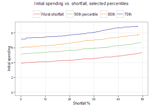
Mapping the initial spending ‘severity frontier’, we see that the highest initial spending with no shortfall is basically the Bengen solution: 3.9% spending, 50% stocks, mostly fixed spending.
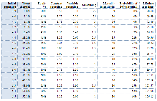
Shortfall: the worst observed decline below initial spending. The ‘frontier’ is the lowest achievable shortfall for an initial spending rate.
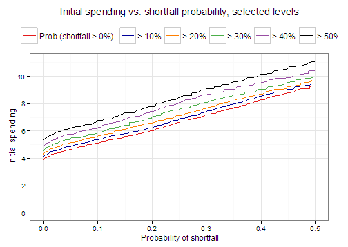
As an aside, below is a plot of probability of shortfall at various levels. Reading across, you can see that at 6%, the best you can do is about a 20% chance of some shortfall and about 4% probability of 50% shortfall (not with identical portfolios). Also, you can see that for each 1% you increase initial spending, best achievable probability of shortfall at any cutoff goes up about 10%.
Mapping the lifetime spending ‘severity frontier’, we see that highest lifetime expected spending with no shortfall is 118.06% of the initial portfolio. This is notably higher than maximizing initial spending with no shortfall. But initial spending is low _ 2.33% of the initial portfolio, which is all equity, like all the other solutions for maximum lifetime spending.
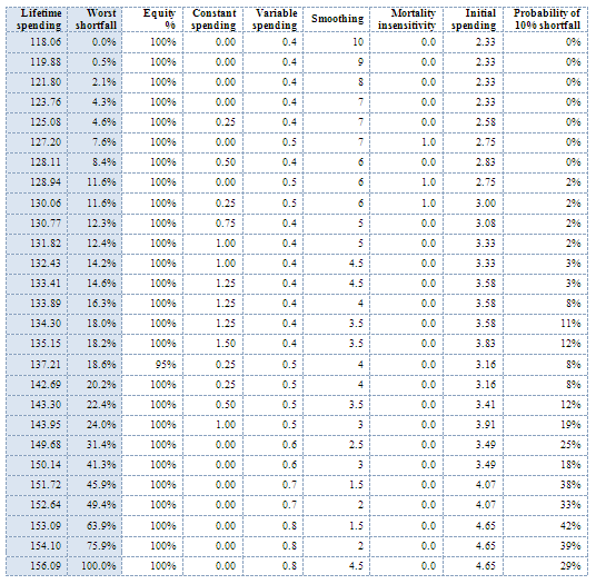
This exposes the essential dilemma::
- If you want maximum initial spending with no shortfall, you have a low-risk portfolio, low lifetime spending. You leave a lot on the table.
- If you want maximum lifetime spending with no shortfall, you have low initial spending, high equity allocation in a portfolio that grows over time and gives you back-loaded spending.
This doesn’t really help us pick an optimal point. We need a ‘Sabermetric’ to combine the ‘holy trinity’ of high spending, low variability, and low risk of shortfall.
There is one in the literature. It’s ‘certainty equivalent’ (CE) spending, which takes an income stream and applies a discount according to 1) its level of variability and risk, and 2) a risk aversion parameter. If risk aversion is 0, you’re risk-neutral, no variability discount is applied. The higher your risk aversion the higher the discount. The form we use is constant relative risk aversion (CRRA), which means a stream that varies between $1 and $2 gets the same discount as one with similar variation between $100 and $200.
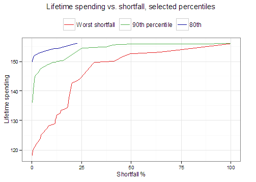
We calculate certainty-equivalent lifetime spending with a risk aversion parameter of 8 _ the lowest that gives us reasonably diversified portfolios. Here is what the ‘severity frontier’ looks like:
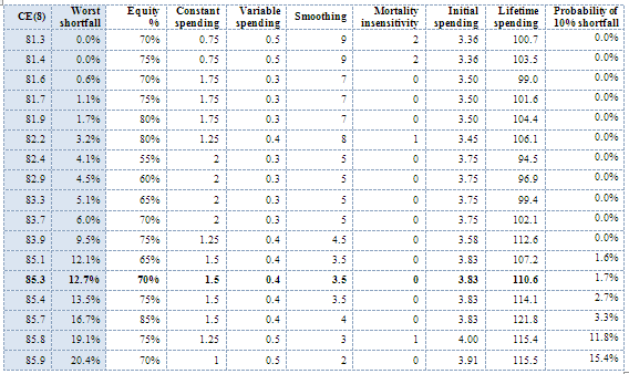
This gives us a higher initial income than maximizing lifetime spending, and a higher lifetime spending than maximizing initial income. For instance, the solution in bold has initial spending of 3.83%, 1.7% probability of shortfall > 10%, lifetime spending > 110% of initial portfolio. Compared to maximizing initial spending for 0 shortfall in Table 1 (3.9% initial spending, 70.7 lifetime spending), we achieve a > 50% increase in lifetime spending at a price of a < 2% decrease in initial spending and a worst-case decline of 12.7% from initial spending. What we find is:
- If we are completely risk neutral, our risk aversion parameter is 0 and we maximize lifetime spending…. we are all equities, low initial spending, high volatility.
- If we are highly risk averse, we will aim for the highest sustainable fixed spending, similar to the Bengen ‘4% rule’.
- If risk aversion is between these two extremes, we will seek a strategy with volatility and lifetime spending between these two extremes. As you increase risk aversion, the variable component of spending decreases and constant spending increases, the portfolio swings from all equities to a diversified mix, and initial spending generally decreases.
If you put full faith in this model and your estimate of risk aversion, you could just maximize certainty-equivalent spending. Or you might want to look up and down the ‘severity frontier’ and pick the best solution, one that combines high lifetime spending and CE spending with reasonable initial spending and shortfall risk.
In practice, maximizing certainty-equivalent spending depends on estimating risk aversion, which is not precisely knowable. We could query retirees on which potential outcomes and risk profiles they prefer, but that’s like describing two movies to them and asking which they would prefer. A portfolio outcome, like a movie, is an experience good, which can only be judged successful after experiencing the whole thing (although failures can often be discovered more quickly, or even from the description). Risk aversion may not even be consistent over time, but may increase abruptly at market extremes.
Nevertheless, certainty-equivalent spending has the advantage of being a consistent, objective measure that takes into account risk and variability, and it can identify a schedule of solutions at different levels of initial and lifetime spending and worst shortfall that are locally optimal, and you can pick the ones that look most desirable.
I wrote this up as a paper with all details, in case others want to delve into it and do more work on it, and will share code and data in this space shortly, as soon as I’ve cleaned it up a little.
I’ll throw out one other approach, which is to use a Kahneman-Tversky behavioral economics/prospect theory utility function, which is discontinuous and heavily penalizes losses from an initial frame of reference. That means it leads to inconsistent choices depending on the initial frame of reference and it’s path-dependent. Yet, it is highly predictive of human choices.
You could apply it to this problem by choosing the highest initial spending such that, if you set it as the initial frame of reference, future utility gains outweigh or equal losses. If you’re highly averse to losses, you’ll set initial spending low enough that the pain from small potential declines in income is offset by very large potential future gains. If you’re less loss averse, you’ll set initial spending a little higher, so moderate losses are offset by large future gains. We still have the thorny problem of estimating the degree of loss aversion. Maybe I’ll do a detailed exploration of that idea, but it might take a while, so I’ll just leave it out there, or if anyone wants to collaborate on a study like that, drop me a line.