Optimal Safe Withdrawal for Retirement Using Certainty-Equivalent Spending, Revisited

Revisiting Bengen’s “4% Rule” at various levels of risk aversion, and generalizing beyond a simple fixed-withdrawal, no-shortfall rule, to flexible rules at different levels of risk aversion.

Disclaimer: this is not investment advice! For educational purposes only. Past performance may not be representative of future results.

A few years ago I was researching withdrawal rates for a relative, and I found the wonderful paper by Bill Bengen on the ‘4% rule.’ The original 4% rule, subsequently updated by Bengen, says that you can invest 50/50 in stocks and bonds, withdraw 4% of your starting portfolio each year of retirement, adjust that number for inflation every year, and in a 30-year retirement, you would never have exhausted your money in any retirement cohort since 1928.

Bengen’s approach finds the highest withdrawal rate subject to a hard no-shortfall constraint.

Then I started thinking, what would happen if, instead of a hard no-shortfall constraint and a fixed withdrawal rate, we asked what flexible rule would maximize spending for different levels of risk aversion?

Using Python, I maximized certainty-equivalent spending, i.e. actual spending discounted by volatility, at different levels of risk aversion, using modern optimization frameworks.

This leads to us to a generalized set of rules, where:

• The Bengen 4% rule is the infinite-risk-aversion solution that requires a fixed constant withdrawal level and never experiences any shortfall or reduction in withdrawals.
• A risk-neutral rule finds the withdrawal amount that historically maximized spending irrespective of volatility, tolerating reductions in spending or shortfalls in some years, as long as they are offset by gains in other years (not recommended for most people).
• In between, different levels of risk aversion lead to different rules that trade off higher mean withdrawals against the risk of lower worst-case withdrawals.

Here are a couple of example results first, and then I’ll explain in more detail what it means, and how it was computed:

A safer rule:

• Allocate 75.20% to stocks. Each year, withdraw 3.54% of starting portfolio + 1.06% of current portfolio.
• Starting spending: 4.60%
• Average spending over 30-year retirement: 5.29% of starting portfolio
• Worst-case spending: 3.58% of starting portfolio

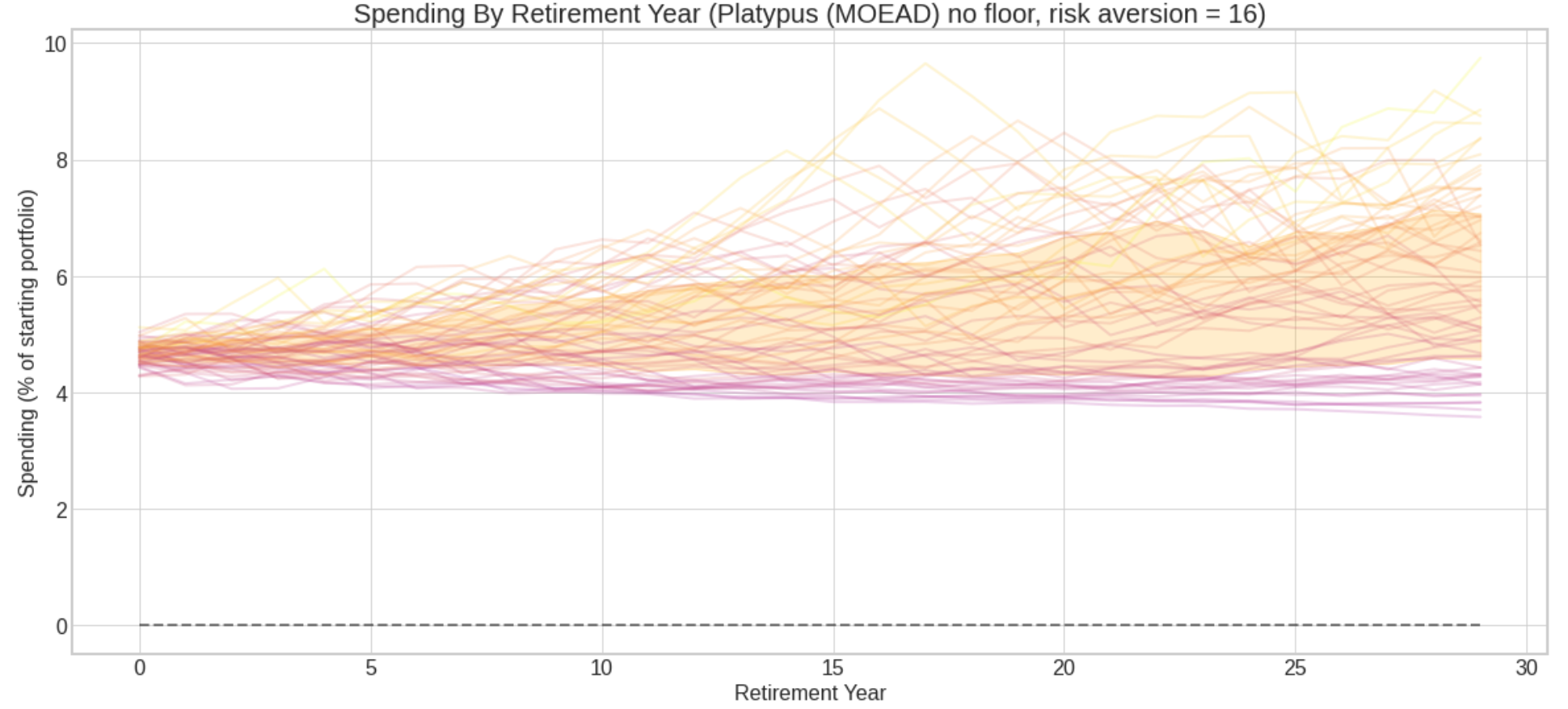
Chart of 30-year spending outcomes of 64 retirement cohorts 1928-1991, risk aversion=16 (Shaded area is middle 50% of outcomes.)

A riskier rule:

• Allocate 87.94% to stocks. Each year, withdraw 2.68% of starting portfolio + 2.96% of current portfolio, or 3.3%, whichever is greater.
• Starting spending: 5.64%
• Average spending over 30-year retirement: 6.87% of starting portfolio
• Worst-case spending: 2.87% of starting portfolio

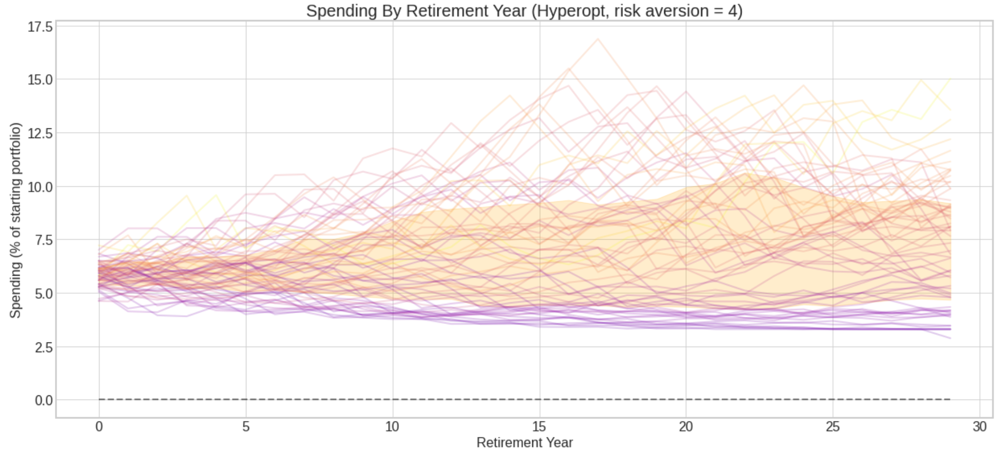
Chart of 30-year spending outcomes of 64 retirement cohorts 1928-1991, risk aversion=4 (Shaded area is middle 50% of outcomes.)

The rules I evaluated work like this:

Asset allocation: Invest a fixed percentage in stocks and bonds, i.e. 60/40. One parameter determines the allocation: stock_alloc, with bond_alloc = 1 - stock_alloc.

Withdrawal: Each year of retirement, withdraw a linear function of the current portfolio, subject to a floor. 3 parameters determine the withdrawal: fixed_pct, variable_pct, floor_pct. Withdraw fixed_pct (intercept), plus portfolio value * variable_pct (slope); or floor_pct, whichever is greater: max(floor_pct, fixed_pct + variable_pct * portval / 100).

Example:

Portfolio value	fixed_pct=2.0	variable_pct=3.0	floor_pct=4.0	Withdrawal
100	2.0	3.0	4.0	5.0
110	2.0	3.3	4.0	5.3
90	2.0	2.7	4.0	4.7
60	2.0	1.8	4.0	4.0

Given these 4 parameters: stock_alloc, fixed_pct, variable_pct, floor_pct, a stream of stock and bond returns, and a starting portfolio, we can calculate how much you would have spent in each year of a 30-year retirement.

And given 64 historical retirement cohorts, we can calculate all the cohort retirement outcomes for a set of parameters, assign a score to each one, and apply an optimization algorithm to find the parameters that yield the best score.

The metric maximized here is certainty-equivalent spending under constant relative risk aversion (CRRA).

CRRA means that you prefer a certain or constant cash stream to a variable or risky one drawn from a distribution; and your preference for similar bets relative to your wealth is invariant as your wealth changes. If I give you a coin-flip with a given positive expected value, for example lose $1/win $2, you will bet the same percentage of your wealth, whether you have $100 or $100,000. And your risk aversion parameter gamma determines whether or how much you choose to bet. If you are risk-neutral you bet more, if you are highly risk-averse, you bet less or refuse the bet.

To calculate certainty-equivalent spending at a level of risk aversion gamma, we convert dollar income streams to the corresponding CRRA utility using gamma. We take the average utility of that income stream, and convert that utility back to dollar spending. This gives us the constant-stream cash flow that would have the same utility as the original variable cash flow at the level of risk aversion represented by gamma.

In essence, we are discounting the cash flows based on their volatility, in the manner implied by CRRA utility. Then, for a given level of risk aversion, we can find the retirement strategy that maximizes certainty-equivalent spending.

I don’t claim that certainty-equivalent spending is a perfect metric to maximize according to any economic theory. But I believe that:

• Certainty-equivalent spending is intuitive: it’s real spending discounted based on volatility and a risk aversion parameter. Units are real dollars. Certainty-equivalent spending is the variable income stream converted to an equivalently desirable constant income stream for a retiree with a given level of risk aversion under CRRA.
• We can, in practice, find strategies that maximize certainty-equivalent spending. Maximizing expected utility directly is more abstract, and can lead to computational and calibration problems.¹
• Certainty-equivalent spending is a quantity that is derived from CRRA utility and consistent with it (even though maximizing expected certainty-equivalent spending over a distribution of returns is not the same as maximizing expected utility).
• Directionally, certainty-equivalent spending is a metric that you could plausibly want to maximize.
• Maximizing certainty-equivalent spending is informative. It allows us to turn a single gamma dial to compute historically optimal parameters for complex strategies at different levels of risk aversion.

If you are making consistent choices, there is some objective function you are maximizing. Certainty-equivalent spending is one possible such objective function, which allows us to compute historically optimal strategies based on the level of risk you are willing to accept. Here is a complete table of results at different levels of risk aversion gamma:

Gamma	Stock %	Fixed %	Variable %	Floor %	Mean Spending %	Worst Case %
0	100.00	0.00	6.31	3.73	8.12	0.00
1	100.00	0.00	6.58	3.43	8.11	2.11
2	98.81	0.69	5.76	3.43	7.97	2.82
4	87.94	2.68	2.96	3.30	6.87	2.87
6	81.77	3.00	2.27	0.00	6.34	3.07
8	78.67	3.19	1.83	0.00	5.98	3.25
10	76.62	3.35	1.49	0.00	5.68	3.39
12	75.94	3.42	1.32	0.00	5.53	3.47
14	75.38	3.50	1.15	0.00	5.38	3.54
16	75.20	3.54	1.06	0.00	5.29	3.58

 

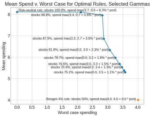
Using some of these rules, a retiree could often have achieved a higher expected withdrawal rate than 4%, at the cost of a modest worsening of the worst-case withdrawal rate. As risk aversion increases, stock allocation decreases, fixed spending increases, and variable spending decreases. The floor parameter is used only at low risk aversion, but may be generally useful in explaining rules. (Or if not, it may be superfluous.)

I don’t assert that one necessarily should maximize certainty-equivalent spending, or that empirically people do try to maximize it. But one could, and it generates a useful menu of strategy choices along a risk continuum.

All models are simplifications, but some are useful. In practice, this framework may allow retirees to visualize and choose between good rules at varying levels of risk tolerance. Knowing that a rule is the best performing according to our metric, and being able to visualize historical performance, may allow retirees to stay the course or make necessary adjustments in adverse environments.

There may be even better parameter setups (glidepaths etc.) and a better objective function to optimize. This general approach can accommodate diferent parameters and objective functions.

In performing this analysis, my goals were:

1) A simple model where we can create understandable strategies that may improve on a fixed withdrawal, at varying levels of risk aversion.

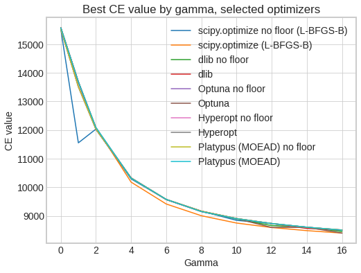
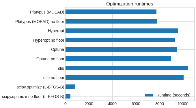
2) To evaluate leading gradient-free optimizing frameworks², including scipy.optimize L-BFGS-B, Optuna, Hyperopt, Platypus, Nevergrad, and Ax. The two that worked best were L-BFGS-B and Optuna, with Dlib, Platypus also yielding useful results. Optimizations were run with and without the floor parameter (‘No floor’: floor fixed at 0). Numerical optimization finds a numerical approximation of the best objective, but we see the optimizers mostly converge to very similar answers, in a reasonable amount of time.

Best objective value found by gamma, selected optimizers:

Optimizer runtimes, selected optimizers (10 runs, 5000 iterations requested, desktop with 12 CPU threads):

3) To build a flexible Python framework for safe withdrawal retirement problems that accomodates:

• Any generator of historical asset returns: historical, Monte Carlo, roll your own market environment as a Python generator function.

• Any asset allocation strategy: fixed weights, glidepath schedules, roll your own based on any parameters.

• Any withdrawal strategy: fixed withdrawal, variable percentage, combinations, glidepaths, any function.

• Any metrics to evaluate retirement cohort outcomes: total spending, certainty-equivalent spending, roll your own. Support survival tables, i.e. calculate expected metric for living retirees taking into account retirement age and survivorship)

• Any (gradient-free) optimizer to find best parameters: e.g. asset allocation, withdrawal parameters to maximize a metric in the given market environment.

Code is found here.

An online tool allowing you to try out and visualize different rules is here.

Additional research that may be pursued within this framework:

• Consider additional asset classes and allocation glidepaths instead of fixed allocations.
• Consider more complex spending rules, such as glidepaths, that change the spending formula over time to allow you to spend more as you get older.
• Instead of fixed 30-year retirements, incorporate an age parameter and mortality curve, and consider only trajectories where the beneficiary is alive.
• Consider bequest utility, add to spending the amount left over at death as equivalent to some fraction of a similar amount of lifetime certainty-equivalent spending.
• Consider other objective functions that can be maximized subject to a risk aversion or loss aversion parameter.
• Compare the recommendations of optimal rules empirically estimated from annual historical returns to recommendations from the formulas derived by Nobel Prize winner Robert C. Merton under continuous-time and lognormal return assumptions, as in “Optimum consumption and portfolio rules in a continuous-time model (1970)” and related papers. (Wikipedia).

Much appreciation to Adam Goldstein and Rudy Beutell for helpful comments and suggestions.

Notes: