‘Cat Food’ revisited – testing dynamic spending rules – Part 2
The last post discussed a framework for evaluating simple dynamic spending rules.
- We defined a spending factor s as spending each year at a rate of s/(remaining life expectancy); and lifetime spending expectancy as the total amount you could expect to spend over your lifetime.
- We showed how, as you increase the spending factor, lifetime spend expectancy initially increases rapidly, but the curve flattens out as spending rate increases.
- We showed how, as you increase the spending factor, shortfall risk initially increases slowly, but the curve steepens as spending rate increases.
We found a simple dynamic spending rule could increase lifetime spending vs. a traditional fixed 4% rule, while keeping shortfall risk relatively low (arguably reducing risk by making the worst case more benign, at the cost of increased volatility, lowered starting spending, higher probability of modest shortfalls).
In this post we’ll look at how smoothing spending can improve outcomes, and how changing the equity/bond mix over time affects outcomes.
Second dynamic rule: Smoothing.
One oddity in Figure 5: even at ultra-low spending rates, you still have a measurable risk of a 25% shortfall from your starting income. At any spending rate, spending is going to vary more or less in line with the market1. So years like 1973 and 1974 might yield big spending drops, even for a 60/40 portfolio at spending rates where you are not at much risk of running out of funds in your lifetime.
If you’re already spending at a low rate, based on a safe long run return expectation, it doesn’t make sense to vary spending exactly in line with a short term change in the markets. And it’s clearly a significant disadvantage over a 4% rule to have that much variation in spending, even when there’s no shortfall.
Let’s introduce smoothing. We’ll still spend at a rate of s/life_expectancy, but instead of multiplying the rate by the latest portfolio value to get spending, we’ll multiply the rate by an exponential moving average2 of the value of previous years’ portfolios.
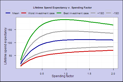
Figure 8. Lifetime spending expectancy (% of initial portfolio) v. spending factor (exponential MA, multiplier 1/3).
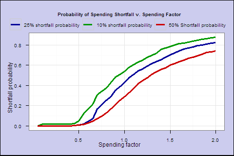
Figure 9. Probability of spending shortfall v. spending factor (exponential MA, multiplier 1/3)
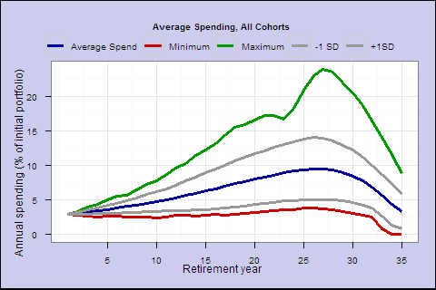
We see a notable improvement _ near 0 shortfall risk out to s of 0.5. As the next chart shows, at s of 0.5, we have slightly higher lifetime spending, smoother overall spending and a better-looking worst case. But, even though overall shortfall probability is much lower, in the worst case you can go broke, if you keep overall spending smooth in the face of a market shortfall very late in life.
Figure 10. Average Spending, All Cohorts (s=0.5, smoothed w/multiplier=1/3)
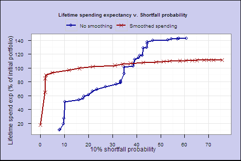
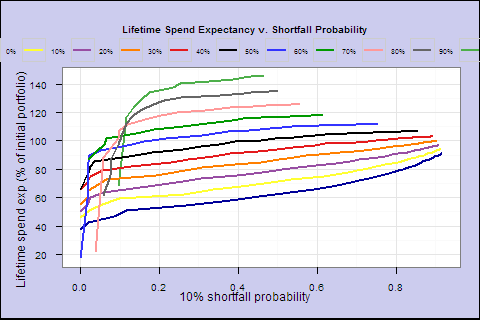
Efficient frontier3. To better visualize the tradeoff, we can combine these 2 graphs into one, which shows the best lifetime spend expectancy we can achieve for any level of shortfall risk:
(‘Efficient frontier’)
For low shortfall rates (the left side), the smoothed spending results in higher lifetime spending expectancy with lower shortfall risk. Smoothing improves the tradeoff, and represents a flexible middle ground between varying spending in line with the market, and setting a fixed spending amount at retirement like the 4% rule.
Portfolio composition
So far, we have looked only at a 60/40 portfolio. Let’s keep the smoothing multiplier at 1/3 and create efficient frontiers for a range of allocations from 0% to 100% stocks.
(‘Efficient frontier’), by % of equities, smoothing multiplier=1/3
We can do this as a big panel (easier to read, esp. the legend): Figure 13. What does this tell us? For this particular smoothing multiplier 1/3, the 50/50 portfolio dominates others (the black line), giving greater lifetime spending at low shortfall probabilities.
Let’s cut to the chase and find for each spending factor, the highest spending expectancy we can achieve with zero shortfall risk, or if zero risk is not feasible, the lowest feasible risk:
|
s |
Life spend expect. |
Prob 10% shortfall |
Prob 25% shortfall |
Prob 50% shortfall |
Equity % |
Smoothing |
| 0.30 | 104.27 | 0.0% | 0.0% | 0.0% | 100% | 5.0 |
| 0.35 | 90.71 | 0.0% | 0.0% | 0.0% | 75% | 4.0 |
| 0.40 | 77.62 | 0.1% | 0.1% | 0.1% | 50% | 3.5 |
| 0.45 | 89.74 | 0.9% | 0.9% | 0.9% | 60% | 4.0 |
| 0.50 | 97.99 | 2.6% | 2.6% | 2.4% | 65% | 4.5 |
| 0.55 | 110.23 | 5.4% | 3.3% | 2.9% | 75% | 4.0 |
| 0.60 | 122.56 | 8.8% | 8.4% | 8.1% | 85% | 6.0 |
| 0.70 | 126.98 | 19.3% | 13.5% | 11.9% | 85% | 5.0 |
| 0.80 | 124.34 | 28.5% | 23.9% | 22.1% | 80% | 6.0 |
| 0.90 | 134.70 | 36.9% | 32.6% | 29.0% | 90% | 6.0 |
| 1.00 | 139.22 | 43.3% | 39.6% | 36.0% | 95% | 6.0 |
</small></center>
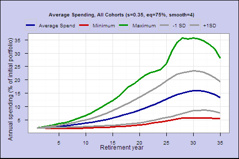
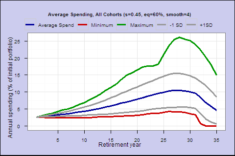
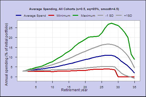
That’s pretty much all we have time for this week. But before we go, let’s look at the spending profiles for 4 solutions.
Spending factor 0.35; Shortfall risk 0%; Lifetime spend expectancy 90.7; Initial spend 2.0%
Spending factor 0.45; Shortfall risk 0.9%; Lifetime spend expectancy 89.7; Initial spend 2.6%
Spending factor 0.5; Shortfall risk 2.6%; Lifetime spend expectancy 98.0; Initial spend 2.9%
Spending factor 0.55; Shortfall risk 5.4%; Lifetime spend expectancy 110.2; Initial spend 3.2%
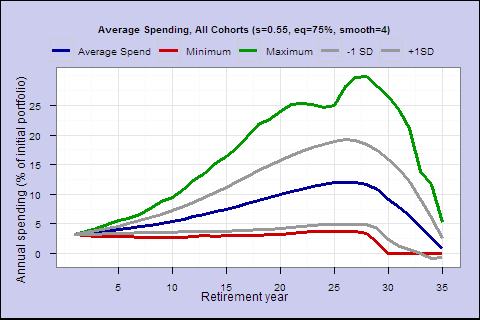
To be 100% safe, we need an initial spending rate below 4% – keeping in mind that the portfolio and spending usually rises over time at safe withdrawal rates. With this restrictive investment universe, the 4% rule is not 100% safe either, and the last chart is a less undesirable spending profile than the 4% fixed spending profile from the last post. On average, total spending is significantly higher, and the worst case is more desirable since it falls short later.
Next time, we’ll look at varying the equity percentage dynamically as you get older, other dynamic rules that might reduce late in life shortfall risk (and the undesirable hump in these curves), and we’ll talk about what the best possible optimal rule would look like.
1modulo the increase in spending rate as you age, from our s/life_expectancy rule. The s spending rate stays the same, but the denominator decreases. </p>
2The exponential moving average has a good combination of sensitivity to the underlying series, and smoothing. A simple n-period moving average, which weights all n periods equally, has undesirable properties. In particular, it’s possible for a simple moving average to move up, when the underlying series is moving below the moving average. Consider this series: 100, 110, 120, 109. A 3-period moving average is after the 3rd element is 110, after the fourth is 113, because the trailing element which left the series (100) is lower than the new element (109).
3This is not exactly the same as the CAPM efficient frontier. For one thing, instead of return, we plot lifetime spending in inflation-adjusted dollars. For another, instead of volatility, it’s the probability of a 25% shortfall from the starting spending. It’s a similar risk v. return plot, but can’t be interpreted quite the same way (eg adding risk-free cash to find additional feasible/optimal portfolios).
</small>
