‘Cat Food’ revisited – testing dynamic spending rules – Part 3
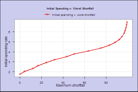
In the last part of our look at dynamic rules for spending in retirement, we discussed how changing the allocation between stocks and bonds affects the maximum sustainable spending rate. We can summarize this relationship by plotting the highest feasible initial spending rate for any acceptable shortfall level.1
equity=0-100%, s=0.05-1.2, smoothing=1.0-6.0)
</p>
| Max shortfall | Init spend % | s | Equity % | Smoothing | Lifetime Spend Exp. |
| 0.0% | 1.7% | 0.30 | 20% | 5 | 58.0 |
| 4.3% | 2.0% | 0.35 | 40% | 4 | 66.3 |
| 12.1% | 2.3% | 0.40 | 50% | 3 | 77.4 |
| 16.9% | 2.6% | 0.45 | 60% | 2.5 | 89.1 |
| 24.7% | 2.9% | 0.50 | 75% | 2 | 105.9 |
| 32.2% | 3.2% | 0.55 | 80% | 1.5 | 113.6 |
| 43.2% | 3.5% | 0.60 | 95% | 1.5 | 132.5 |
| 50.4% | 3.8% | 0.65 | 95% | 1 | 133.8 |
| 63.5% | 4.1% | 0.70 | 100% | 1 | 141.0 |
</small></center>
In part 3 today, we’re going to discuss 1) adding a parameter to change the way we increase the spending rate as we get older and 2) reducing equity allocation as we get older. Finally, we’re going to do a brute-force search for the highest initial spending and best parameters for each level of shortfall risk (skip to conclusion).
Adjusting how fast spending rate increases with age
Suppose we are willing to accept the portfolio in bold and spending rate, which has never resulted in a decline greater than 24.7% below the initial spending amount. We use spending factor s=0.5, equity = 75%, smoothing factor = 2. We end up with a spending profile that looks like this:
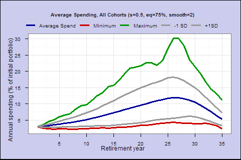
Notice the ‘hump.’ In the average case, spending rises steadily, then drops. Ideally, we would like a flatter spending profile, preferring less variability in spending. If we could take the hump and spread part of it earlier, without increasing shortfall risk, it would increase the safe spending rate.
The spending rate at age 99 is s/life_expectancy=0.5/2.19 = 22.8%. Spending rates at advanced ages are too high, decimating the portfolio and causing the decline in spending. If we reduce them, maybe we don’t need to build as big a war chest in middle years to support such a high spending rate in late years.
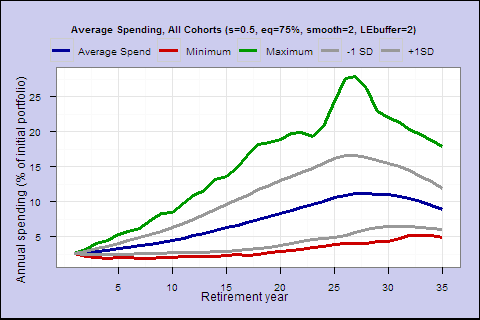
There are several ways we could change the model to flatten the spending profile. The one we choose is to add a parameter we’ll call ‘life expectancy buffer’ to life expectancy, so we’ll spend at a rate of s/(life_expectancy+buffer). If the parameter is 2, then when our life expectancy is 3, instead of spending at a rate of s/3, we’ll spend at a rate of s/(3+2). If life expectancy buffer is 0 or low, the spending rate will rise relatively quickly as we age; if life expectancy buffer is large, the spending rate will change slowly as we age.
With a buffer of 2, we get a flatter spending profile later in life, without changing too much at the start of retirement.
Let’s compare efficient frontiers, with and without the buffer:
Buffer=1 v. Buffer=0
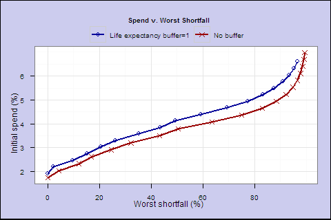
We find in all cases, the buffer gives us a higher level of initial spending for any level of shortfall risk. However, increasing the buffer does not always increase lifetime spending and sometimes worsens the tradeoff.
Buffer=1 v. Buffer=0
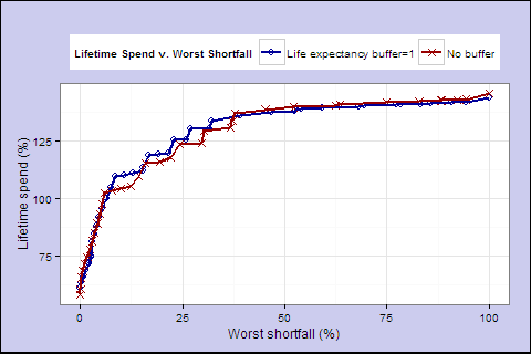
It’s a mixed picture. The buffer may in many cases allow us to spend safely at a higher initial rate, but doesn’t always improve lifetime spending. Sometimes it reduces portfolio growth and overall lifetime spending.
Third dynamic rule: Changing equity allocation over time.
Does it make sense to reduce the equity allocation as you get older? Let’s introduce a variable to gradually reduce the amount of equity. As long as your life expectancy is > 15 years, use the initial allocation. After that, we’ll reduce the equity percentage by stepdown percentage points per year.
Equity stepdowns from 0 to 3% per year when LE<15 years.
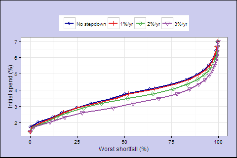
Equity stepdowns from 0 to 3% per year.
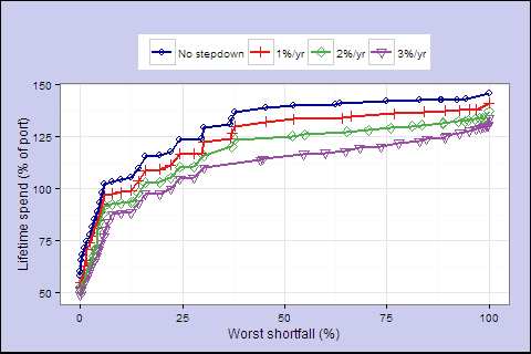
What I thought would happen: stepping down equity over time would let you start with more equity, relying on smoothing to get you over early drawdowns and strong long-run real returns to catch up. Then with lower equity in later years you wouldn’t be exposed to big drawdowns late in life.
What actually happened: stepping down equities always worsens the risk/reward tradeoff.
Apparently my preconception was faulty, or this is the wrong model, stepping down too early and killing returns, or there’s a mistake somewhere (although I don’t think so). Watch this space for possible future elaboration or ninja-edit. I’ll consider this a first draft and move on.
Discarding the stepdown, we now have 4 parameters: spending factor s, starting equity, smoothing factor, and lifetime buffer. We have discussed how each one impacts the spending profile and shortfall risk. Let’s put it all together, try running a full range of reasonable values, and come up with the best efficient frontier over all values.
(s=.05-1.2; equity=0-100%; smooth=1-6; buffer=0-5)
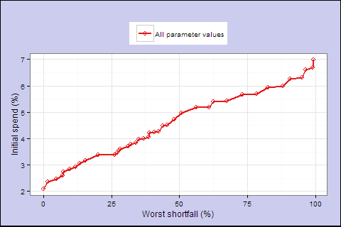
</p>
| Max shortfall | Init spend % | s | Equity % | Smoothing | Buffer | Lifetime Spend Exp. |
| 0.0% | 2.1% | 0.40 | 20% | 6.0 | 2 | 55.5 |
| 1.6% | 2.3% | 0.45 | 35% | 6.0 | 2 | 64.4 |
| 4.8% | 2.5% | 0.50 | 40% | 6.0 | 3 | 66.9 |
| 7.2% | 2.6% | 0.55 | 40% | 6.0 | 4 | 67.18 |
| 7.4% | 2.7% | 0.55 | 55% | 6.0 | 3 | 79.0 |
| 9.8% | 2.8% | 0.60 | 55% | 6.0 | 4 | 78.7 |
| 11.8% | 2.9% | 0.65 | 55% | 6.0 | 5 | 78.5 |
| 13.4% | 3.1% | 0.65 | 75% | 6.0 | 4 | 95.3 |
| 15.4% | 3.2% | 0.70 | 75% | 6.0 | 5 | 94.6 |
| 20.1% | 3.4% | 0.75 | 95% | 6.0 | 5 | 114.1 |
| 27.3% | 3.5% | 0.70 | 90% | 3.5 | 3 | 117.6 |
| 27.8% | 3.5% | 0.75 | 80% | 3.5 | 4 | 106.7 |
| 28.4% | 3.6% | 0.80 | 85% | 4.0 | 5 | 109.7 |
| 31.0% | 3.7% | 0.75 | 75% | 2.5 | 3 | 106.2 |
| 32.3% | 3.8% | 0.80 | 85% | 3.0 | 4 | 113.8 |
| 34.0% | 3.8% | 0.85 | 90% | 3.5 | 5 | 117.1 |
| 35.1% | 4.0% | 0.80 | 95% | 2.5 | 3 | 127.8 |
| 37.0% | 4.0% | 0.85 | 90% | 2.5 | 4 | 120.8 |
| 38.6% | 4.1% | 0.90 | 90% | 3.0 | 5 | 119.4 |
| 39.0% | 4.2% | 0.85 | 95% | 2.0 | 3 | 129.3 |
| 40.7% | 4.2% | 0.90 | 95% | 2.0 | 4 | 127.6 |
| 42.3% | 4.3% | 0.95 | 90% | 2.5 | 5 | 121.2 |
| 44.0% | 4.5% | 0.95 | 100% | 2.0 | 4 | 134.5 |
| 45.5% | 4.5% | 1.00 | 100% | 2.0 | 5 | 132.9 |
| 48.1% | 4.7% | 1.05 | 95% | 1.5 | 5 | 128.6 |
| 50.6% | 5.0% | 1.10 | 100% | 1.5 | 5 | 134.8 |
</small>
Let’s look at the rule in bold. (s=0.70, equity=75%, smooth=6.0, buffer=5)
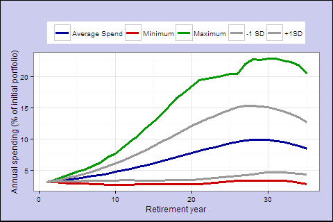
</center>
What have we learned?
- When you retire matters. A lot.
- The 4% rule doesn’t really work with a restrictive large cap/long term bond portfolio. The best solution is 95% equity and you still get a worst case 35% shortfall.
- < 3.5% has generally had a tolerable worst-case, and on average lets your spending grow over time to > 4% of the initial portfolio.
- Even at 3.2-3.5%, a dynamic rule gives you higher lifetime spending than a fixed 4% rule, and the failure scenarios are gradual, not sudden and catastrophic.
- A large equity allocation is desirable for real long-term growth, and stepping down the amount of equity as you get older doesn’t seem to improve risk-reward (at least, not a fixed annual stepdown when life expectancy is < 15 years).
- Taxes and investment expenses aren’t included and must be taken into account, reducing returns and the level of safe spending.
- On the other hand, including higher-risk, higher-return investments, like small caps, international equities, higher-yielding bonds should improve risk-reward and allow higher returns and spending.
- Of course, this analysis assumes the future will not be very different from the past.
- Finally, I would add that life annuities, in theory, could be a free lunch. In the analysis above, you put aside 100% of the money you may need in the 25% chance you live to be 90; alternatively, you could join an annuity pool which only needs to put aside money for the survivors, which also has tax advantages. However, fixed annuities are subject to inflation and credit risk, and the market for insurance products for the elderly is a jungle teeming with predators.
These dynamic rules are chosen for analytical simplicity, to be easy to understand and calculate. There’s no reason to believe that they are the best, ie spending a constant/(life expectancy+buffer) is the ideal model to get the highest spending rate at each point in time for the lowest shortfall risk.
In the last part of this series, we’ll think about what an ideal model would look, and how to maximize spending while keeping shortfall risk at an acceptable level.
1On further review, the table in Part 2 isn’t the best way to look at it. No one thinks about the best spending factor they can achieve, they think about the initial spending %. And people don’t think about ‘lowest probability of 10% shortfall.’ Maximum acceptable shortfall is simpler and more informative.