A Piketty counterargument: Is r > g a reasonable assumption?
A thought experiment: If you could buy an asset that returned the GDP growth rate, would you, should you do it?
In other words, if you had a choice of Piketty’s r and g, from his ‘Iron Law’ equation r > g, which would you choose?
Marc Andreessen said, “The funny thing about Piketty is that he has a lot more faith in returns on invested capital than any professional investor I’ve ever met.” And I tend to agree with him. If someone offered me a guarantee of g, I would put a good chunk of my retirement portfolio into it.
Why?
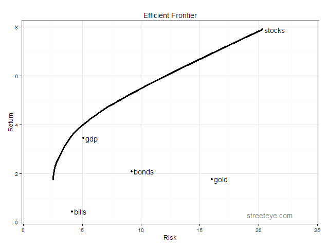
- US real GDP growth has averaged about 3.5% since 1930.
- Bonds’ long run real returns are less than GDP growth, maybe 2% real (and remarkably less right now).
- Stocks return more historically: on average about 8% real returns since 1930. (and also currently priced to underperform)
- But stock returns are super bumpy. In 2008 they were down 37% on the year (and more at the trough).
- Companies have financial and operating leverage, so in the medium term stocks are like an option on GDP struck at expected GDP. If GDP outperforms the expectations built into prices when you buy stocks, you’ll do really well, if GDP disappoints, you will lose quite a bit of money.
- In the longer run, the outperformance of stocks over GDP seems to stem from 1) more leverage/risk and 2) historically, persistently better than expected outcomes, which is another way of saying a persistently excessive equity risk premium. People have historically feared stock volatility even more than they reasonably should have feared those 37% crashes, or stocks and the economy have historically on average outperformed people’s expectations.
- The r Piketty refers to is the unlevered real return across all deployments of capital in GDP: Residential, non-residential construction, plant and equipment, inventories/working capital. 1
We can compute, historically, if g would have offered a good deal within the major investment classes. So let’s try it! Using historical real returns of US stocks, bonds, bills, gold, and this hypothetical GDP asset, the efficient frontier looks like this:
And the transition map showing the efficient portfolio: As you go from left to right, you increase your risk and return, move out on the efficient frontier, and the composition of your portfolio changes.
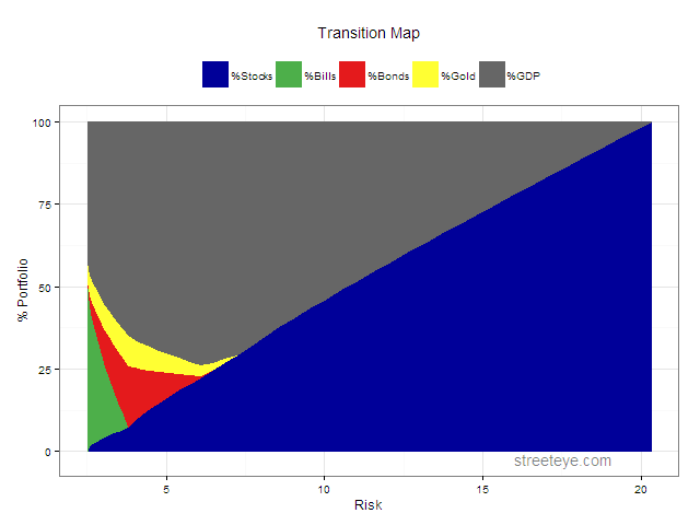
The minimum risk portfolio starts with about 40% GDP. As you stretch for higher risk and returns it peaks at about 75%, before giving way to an increasing mix of higher returning stocks.
The bottom line is, if you could buy g, in most cases you would devote quite a big chunk of your portfolio to it. All the portfolios we would consider diversified have more ‘GDP’ than stocks.
Piketty makes the following claims:
- When the rate of return on capital r is greater than the rate of GDP growth g, owners of capital get richer faster than wage-earners.
- It is an ‘iron law of capitalism’ that in that situation inequality will increase.
- This is a problem, and to avoid the ills associated with that, a global capital levy is an appropriate solution.
I would make the following counterclaims:
- If people could buy an asset with r=g, they would.
- If some people could persistently identify assets and strategies that earned r>g, they could make money supplying GDP-linked bonds or swaps which paid g, turn around and invest at r>g and make a profit.
- We don’t see this sort of profitable banking or arbitrage in the marketplace. Even Warren Buffett wouldn’t offer g-linked bonds in size. Why not? Because he can put his hands on cash at better terms. And because if someone had offered such a deal at the beginning of 1930 (never mind the stock market peak) and invested in stocks, they wouldn’t have broken even until the 50s. And bonds don’t save you due to their low returns.
It seems to me the market is telling us it does not believe r > g.
r seems partly endogenous and partly exogenous: it depends on availability of capital and the return on the available investment opportunities, which can also be highly uncertain and idiosyncratic.
As a thought experiment, suppose cheap fusion was invented tomorrow. That would result in an investment boom. Enterprises making fusion reactors, fusion vehicles, all manner of cheap fusion energy-powered factories would suck in capital, crowd out other investments, r would go up, and an era of plenty for mankind would hopefully ensue as all those investments threw off great r initially, and eventually g. r would presumably rise above g initially, and then fall below it as the big rise in g threw off more surplus investment capital than people knew what to do with. That’s what boom/busts generally look like.
On the other hand, if oil suddenly runs out, or California tumbles into the Pacific, r will be negative, a lot of people with large capital investments will find them uneconomic, or lose them entirely to the whims of fate.
If you combine all the layers of the economy’s capital structure, including residential, non-residential structures and plant and equipment, working capital/inventories, I think the safer bet in the very long run is r ~= g. Piketty shows anything else is unsustainable. If r < g, there is too much capital and investors are foolishly investing in poor projects that lose money and the economy is getting less and less capital intensive over time. If there were no countervailing forces, this would presumably continue, until we’re back to performing surgery with stone knives and bear skins. If r > g, the economy is getting more capital-intensive over time, investors are under-investing in given growth opportunities due to scarcity of capital. If you believe Piketty, this continues until you somehow end up with a few capitalist lords supervising armies of robots and starving serfs.
Over the very long run, I don’t see any reason to think either situation qualifies as ‘iron law’. If anything the capitalist era has seen wealth distributed more widely than in the feudal era, and after a few hundred years we’re not once again ruled by a few kings and armies of serfs and robots (although recent tendencies in that direction are a bit concerning).
As an accounting identity you can say, when r>g, capital owners are doing better than everyone else.
You just can’t turn that into a statement about perpetually increasing inequality without heroic assumptions about how capital is distributed, and how the distribution of capital income, and wage income is changing. (Including how new wealth destroys old wealth, e.g. Apple destroys RIM and Nokia, how wealth gets dispersed over generations, how it eventually falls into the hands of fools and gets destroyed and dissipated.)
If that isn’t enough, let me throw out one more, entirely unrelated point. The distinction between return on capital and return on labor is ultimately more fuzzy and arbitrary than one might think.
Mitt Romney made a modest fortune from Bain Capital. Not only did he benefit from getting paid in ‘carried interest’ which was taxed as a capital gain at 15%, but he also put the most levered bets into his IRA, where they appreciated with no tax hit at all, until he decides to withdraw them.
Of course, if IRAs don’t get taxed, and capital gains are taxed at 15% instead of 39.6% on income, no one can blame him for structuring his compensation as capital gains.
And can anyone argue that if the tax rates were reversed, the payout would have come as bonuses and labor income for his talents and hard work, not as capital gains?
The distinction between return on capital and labor is in large part arbitrary when it comes to the top 1%. Whether you own a hot dog stand, a medical practice, or are a founder of Microsoft, it’s pretty much impossible to tell which part of the income is from your hard work and which is a return on investment from…your hard work in earlier years. And it’s a little pointless to try.
Goodhart’s Law: ‘Iron laws’ turn out to be made of straw once you depend on them for policy outcomes.
Democratic societies are founded on equality of opportunity, equality before the law, equality in the voting booth. When so much of our life takes place in the economic sphere, excessive inequality of wealth and income inevitably leads to inequality of opportunity and inequality before the law. r > g, the “iron law” and the global wealth tax, are an academic sideshow, and taken to an extreme, divorced from reality and common sense. We should strive for better education and opportunity for everyone, and a fairer tax system than the current abomination. Bill Gates has a thoughtful perspective on the subject, noteworthy because of where his own personal interests lie.
1 It’s a bit challenging to calculate the unlevered returns to all the capital deployed in GDP, but that hasn’t stopped some from trying. Logically, that rate of return should be in the realm of returns available from the universe of investable securities, after expenses, if for no other reason than that companies can issue stocks and bonds to fund capital projects, and when market rates are low and project returns are high, they will issue securities and fund projects until the gap no longer provides that incentive. In any event, that universe of securities represents the investments generally available to all those capital owners Piketty thinks have the tendency to get richer and richer.
2Let’s try anyway. In the case of the hot-dog vendor, you can ask what the cart-owner would have to pay to hire someone at salary to sell the dogs and say the balance is return on capital. But the wage-earner won’t work as hard and sell as many. Some of the difference is because the owner is in fact working harder. Same applies to the CEO. Bill Gates could have paid someone else to be CEO. But Microsoft wouldn’t have done as well. It’s quite hard to say how much of the money he made, or any of the Microsoft millionaires for that matter, was labor income, and how much was return on income foregone and re-invested in the company.
install.packages('lpSolve') require(lpSolve) install.packages('quadprog') require(quadprog) require(ggplot2) require("reshape") SP500 = c(-0.2512,-0.4384,-0.0864,0.4998,-0.0119,0.4674,0.3194,-0.3534,0.2928,-0.011,-0.1067,-0.1277,0.1917,0.2506,0.1903,0.3582,-0.0843,0.052,0.057,0.183,0.3081,0.2368,0.1815,-0.0121,0.5256,0.326,0.0744,-0.1046,0.4372,0.1206,0.0034,0.2664,-0.0881,0.2261,0.1642,0.124,-0.0997,0.238,0.1081,-0.0824,0.0356,0.1422,0.1876,-0.1431,-0.259,0.37,0.2383,-0.0698,0.0651,0.1852,0.3174,-0.047,0.2042,0.2234,0.0615,0.3124,0.1849,0.0581,0.1654,0.3148,-0.0306,0.3023,0.0749,0.0997,0.0133,0.372,0.2382,0.3186,0.2834,0.2089,-0.0903,-0.1185,-0.2197,0.2836,0.1074,0.0483,0.1561,0.0548,-0.3658,0.2592,0.1486) BONDS = c(0.0454,-0.0256,0.0879,0.0186,0.0796,0.0447,0.0502,0.0138,0.0421,0.0441,0.054,-0.0202,0.0229,0.0249,0.0258,0.038,0.0313,0.0092,0.0195,0.0466,0.0043,-0.003,0.0227,0.0414,0.0329,-0.0134,-0.0226,0.068,-0.021,-0.0265,0.1164,0.0206,0.0569,0.0168,0.0373,0.0072,0.0291,-0.0158,0.0327,-0.0501,0.1675,0.0979,0.0282,0.0366,0.0199,0.0361,0.1598,0.0129,-0.0078,0.0067,-0.0299,0.082,0.3281,0.032,0.1373,0.2571,0.2428,-0.0496,0.0822,0.1769,0.0624,0.15,0.0936,0.1421,-0.0804,0.2348,0.0143,0.0994,0.1492,-0.0825,0.1666,0.0557,0.1512,0.0038,0.0449,0.0287,0.0196,0.1021,0.201,-0.1112,0.0846) BILLS = c(0.0455,0.0231,0.0107,0.0096,0.0032,0.0018,0.0017,0.003,0.0008,0.0004,0.0003,0.0008,0.0034,0.0038,0.0038,0.0038,0.0038,0.0057,0.0102,0.011,0.0117,0.0148,0.0167,0.0189,0.0096,0.0166,0.0256,0.0323,0.0178,0.0326,0.0305,0.0227,0.0278,0.0311,0.0351,0.039,0.0484,0.0433,0.0526,0.0656,0.0669,0.0454,0.0395,0.0673,0.0778,0.0599,0.0497,0.0513,0.0693,0.0994,0.1122,0.143,0.1101,0.0845,0.0961,0.0749,0.0604,0.0572,0.0645,0.0811,0.0755,0.0561,0.0341,0.0298,0.0399,0.0552,0.0502,0.0505,0.0473,0.0451,0.0576,0.0367,0.0166,0.0103,0.0123,0.0301,0.0468,0.0464,0.0159,0.0014,0.0013) CPI = c(-0.0639535,-0.0931677,-0.1027397,0.0076336,0.0151515,0.0298507,0.0144928,0.0285714,-0.0277778,,0.0071429,0.0992908,0.0903226,0.0295858,0.0229885,0.0224719,0.1813187,0.0883721,0.0299145,-0.0207469,0.059322,0.06,0.0075472,0.0074906,-0.0074349,0.0037453,0.0298507,0.0289855,0.0176056,0.017301,0.0136054,0.0067114,0.0133333,0.0164474,0.0097087,0.0192308,0.0345912,0.0303951,0.0471976,0.0619718,0.0557029,0.0326633,0.0340633,0.0870588,0.1233766,0.0693642,0.0486486,0.0670103,0.0901771,0.1329394,0.125163,0.0892236,0.0382979,0.0379098,0.0394867,0.0379867,0.010979,0.0443439,0.0441941,0.046473,0.0610626,0.0306428,0.0290065,0.0274841,0.026749,0.0253841,0.0332248,0.017024,0.016119,0.0268456,0.0338681,0.0155172,0.0237691,0.0187949,0.0325556,0.0341566,0.0254065,0.0408127,0.0009141,0.0272133,0.0149572) GOLD = c(,,,0.44700286,0.079661828,,,,,,-0.014388737,0.028573372,,0.027779564,-0.006872879,0.027212564,0.026491615,0.117056555,-0.023530497,-0.036367644,-0.00619197,-0.00623055,-0.033039854,-0.086306904,-0.007067167,-0.002840911,0.001421464,0.001419447,,,0.034846731,-0.027779564,-0.004234304,-0.002832863,0.002832863,0.004234304,-0.002820876,0.002820876,0.203228242,-0.059188871,-0.052577816,0.136739608,0.358646094,0.511577221,0.545727802,-0.132280611,-0.253090628,0.168898536,0.265477915,0.464157559,0.689884535,-0.285505793,-0.201637346,0.120144312,-0.163629424,-0.127202258,0.149181164,0.192236014,-0.020385757,-0.134512586,0.005221944,-0.058998341,-0.051002554,0.045462374,0.064538521,0.002600782,0.010336009,-0.155436854,-0.121167134,-0.052185753,,-0.028987537,0.133990846,0.157360955,0.119003292,0.084161792,0.308209839,0.142551544,0.220855221,0.110501915,0.228258652) GDP = c(-0.085084232,-0.064032275,-0.128868258,-0.012560264,0.107799049,0.089074461,0.129392971,0.051013673,-0.033106047,0.079706783,0.08808869,0.17707922,0.188888143,0.170391692,0.079905483,-0.009645441,-0.115835513,-0.010964353,0.041559245,-0.00549505,0.087162129,0.080586081,0.040720339,0.046944343,-0.005638952,0.071219054,0.02132165,0.021055266,-0.007352169,0.069022678,0.025635104,0.025541223,0.061164957,0.043539949,0.057670519,0.064997322,0.065934066,0.027436363,0.049090742,0.03140731,0.002015915,0.032952139,0.052628342,0.056443916,-0.005180583,-0.001964418,0.053849296,0.046093667,0.055617315,0.031752617,-0.002443475,0.025936376,-0.019100292,0.046323541,0.072585395,0.042388469,0.035120756,0.034616119,0.042040676,0.036804531,0.019188746,-0.000737018,0.03555943,0.027453435,0.04037391,0.027197286,0.03795652,0.044872645,0.044495193,0.046851005,0.040925252,0.009753418,0.017867562,0.028066125,0.037856696,0.033448288,0.026668165,0.01778456,-0.002911179,-0.027760546,0.025321284) # put into a data frame (matrix) fnominal=data.frame(stocks=SP500, bills=BILLS, bonds=BONDS, gold=GOLD, CPI=CPI, GDP=GDP) freal=data.frame(stocks=SP500-CPI, bills=BILLS-CPI, bonds=BONDS-CPI, gold=GOLD-CPI, gdp=GDP) # compute means realreturns = apply(freal, 2, mean) realreturnspct = realreturns*100 # print them realreturnspct # compute sds realsds = apply(freal, 2, sd) realsdspct = realsds*100 # print them realsdspct # find maximum return portfolio (rightmost point of efficient frontier) # will be 100% of highest return asset # maximize # w1 * stocks +w2 *bills +w3*bonds + w4 * gold # subject to 0 <= w <= 1 for each w # will pick highest return asset with w=1 # skipping >0 constraint, no negative return assets, so not binding opt.objective <- realreturns opt.constraints <- matrix (c(1, 1, 1, 1, 1, # constrain sum of weights to 1 1, , , , , # constrain w1 <= 1 , 1, , , , # constrain w2 <= 1 , , 1, , , # constrain w3 <= 1 , , , 1, , # constrain w4 <= 1 , , , , 1), # constrain w5 <= 1 nrow=6, byrow=TRUE) opt.operator <- c("=", "<=", "<=", "<=", "<=", "<=") opt.rhs <- c(1, 1, 1, 1, 1, 1) opt.dir="max" solution.maxret = lp (direction = opt.dir, opt.objective, opt.constraints, opt.operator, opt.rhs) # portfolio weights for max return portfolio wts.maxret=solution.maxret$solution # return for max return portfolio ret.maxret=solution.maxret$objval # compute return covariance matrix to determine volatility of this portfolio covmatrix = cov(freal, use = 'complete.obs', method = 'pearson') # multiply weights x covariances x weights, gives variance var.maxret = wts.maxret %*% covmatrix %*% wts.maxret # square root gives standard deviation (volatility) vol.maxret = sqrt(var.maxret) wts.maxret ret.maxret vol.maxret ################################################################################ # find minimum volatility portfolio (leftmost point of efficient frontier) covmatrix = cov(freal, use = 'complete.obs', method = 'pearson') nObs <- length(freal$stocks) nAssets <- length(freal) # 1 x numassets array of 1s opt.constraints <- matrix (c( 1, 1, 1, 1, 1, # sum of weights =1 1, , , , , # w1 >= 0 , 1, , , , # w2 >= 0 , , 1, , , # w3 >= 0 , , , 1, , # w4 >= 0 , , , , 1 # w5 >= 0 ) , nrow=6, byrow=TRUE) opt.rhs <- matrix(c(1, 0.000001, 0.000001, 0.000001, 0.000001, 0.000001)) opt.meq <- 1 # first constraint is '=', rest are '>=' zeros <- array(, dim = c(nAssets,1)) solution.minvol <- solve.QP(covmatrix, zeros, t(opt.constraints), opt.rhs, meq = opt.meq) wts.minvol = solution.minvol$solution var.minvol = solution.minvol$value *2 ret.minvol = realreturns %*% wts.minvol vol.minvol = sqrt(var.minvol) ################################################################################ # generate a sequence of 50 evenly spaced returns between min var return and max return lowreturn=ret.minvol highreturn=ret.maxret minreturns=seq(lowreturn, highreturn, length.out=50) # add a return constraint: sum of weight * return >= x retconst= rbind(opt.constraints, realreturns) retrhs=rbind(opt.rhs, ret.minvol) # create vectors for the returns, vols, and weights along the frontier, # starting with the minvol portfolio out.ret=c(ret.minvol) out.vol=c(vol.minvol) out.stocks=c(wts.minvol[1]) out.bills=c(wts.minvol[2]) out.bonds=c(wts.minvol[3]) out.gold=c(wts.minvol[4]) out.gdp=c(wts.minvol[5]) # loop and run a minimum volatility optimization for each return level from 2-49 for(i in 2:(length(minreturns) - 1)) { print(i) # start with existing constraints, no return constraint tmp.constraints = retconst tmp.rhs=retrhs # set return constraint tmp.rhs[7] = minreturns[i] tmpsol <- solve.QP(covmatrix, zeros, t(tmp.constraints), tmp.rhs, meq = opt.meq) tmp.wts = tmpsol$solution tmp.var = tmpsol$value *2 out.ret[i] = realreturns %*% tmp.wts out.vol[i] = sqrt(tmp.var) out.stocks[i]=tmp.wts[1] out.bills[i]=tmp.wts[2] out.bonds[i]=tmp.wts[3] out.gold[i]=tmp.wts[4] out.gdp[i]=tmp.wts[5] } # put maxreturn portfolio in return series for max return, index =50 out.ret[50]=c(ret.maxret) out.vol[50]=c(vol.maxret) out.stocks[50]=c(wts.maxret[1]) out.bills[50]=c(wts.maxret[2]) out.bonds[50]=c(wts.maxret[3]) out.gold[50]=c(wts.maxret[4]) out.gdp[50]=c(wts.maxret[5]) # organize in a data frame efrontier=data.frame(out.ret*100) efrontier$vol=out.vol*100 efrontier$stocks=out.stocks*100 efrontier$bills=out.bills*100 efrontier$bonds=out.bonds*100 efrontier$gold=out.gold*100 efrontier$gdp=out.gdp*100 names(efrontier) = c("Return", "Risk", "%Stocks", "%Bills", "%Bonds", "%Gold", "%GDP") ################################################################################ # define colors dvblue = "#000099" dvred = "#e41a1c" dvgreen = "#4daf4a" dvpurple = "#984ea3" dvorange = "#ff7f00" dvyellow = "#ffff33" dvgray="#666666" apoints=data.frame(realsdspct) apoints$realreturns = realreturnspct ggplot(data=efrontier, aes(x=Risk, y=Return)) + opts(title="Efficient Frontier") + theme_bw() + geom_line(size=1.4) + geom_point(aes(x=apoints$realsdspct, y=apoints$realreturns)) + scale_x_continuous(limits=c(1,24)) + annotate("text", apoints[1,1], apoints[1,2],label=" stocks", hjust=) + annotate("text", apoints[2,1], apoints[2,2],label=" bills", hjust=) + annotate("text", apoints[3,1], apoints[3,2],label=" bonds", hjust=) + annotate("text", apoints[4,1], apoints[4,2],label=" gold", hjust=) + annotate("text", apoints[5,1], apoints[5,2],label=" gdp", hjust=) + annotate("text", 19,0.3,label="streeteye.com", hjust=, alpha=0.5) ################################################################################ keep=c("Risk", "%Stocks","%Bills","%Bonds","%Gold", "%GDP") efrontier.tmp = efrontier[keep] efrontier.m = melt(efrontier.tmp, id ='Risk') ggplot(data=efrontier.m, aes(x=Risk, y=value, colour=variable, fill=variable)) + theme_bw() + opts(title="Transition Map", legend.position="top", legend.direction="horizontal") + ylab('% Portfolio') + geom_area() + scale_colour_manual("", breaks=c("%Stocks", "%Bills", "%Bonds","%Gold","%GDP"), values = c(dvblue,dvgreen,dvred,dvyellow,dvgray), labels=c('%Stocks', '%Bills','%Bonds','%Gold','%GDP')) + scale_fill_manual("", breaks=c("%Stocks", "%Bills", "%Bonds","%Gold","%GDP"), values = c(dvblue,dvgreen,dvred,dvyellow,dvgray), labels=c('%Stocks', '%Bills','%Bonds','%Gold','%GDP')) + annotate("text", 16,-2.5,label="streeteye.com", hjust=, alpha=0.5) |