Safe Retirement Spending Using Certainty Equivalent Values and TensorFlow
Certainty equivalent value is the concept of applying a discount to a stream of cash flows based on how variable or risky the stream is…like the inverse function of the risk premium.
TensorFlow is a machine learning framework that Google released last November 2015. TensorFlow is a powerful tool to find optimal solutions to machine learning problems, like neural networks in Google’s search platform.1
Building on these concepts previously presented in my article for AAII on Safe Withdrawal Rates and Certainty-Equivalent Spending, in this post we’ll construct optimized asset allocations and withdrawal plan for retirement using TensorFlow.
It’s an interesting problem; maybe it’s an interesting and/or original solution, and if nothing else it’s a starter code example for how one can use TensorFlow to solve an optimization problem like this.
This is not investment advice! This is a historical study/mad science experiment. It may not be applicable to you, it is a work in progress, and it may contain errors.
1) The solution.
To cut to the chase, here is an estimate of the asset allocation and spending plan for a 30-year retirement, that would have maximized certainty-equivalent cash flow for a somewhat risk-averse retiree over the last 59 years:
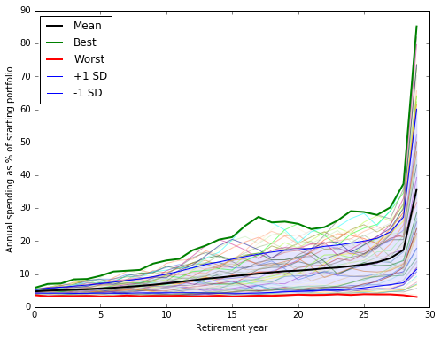
Spending paths, 30-year retirements, 1928-1986, γ = 8
The black line is the mean outcome. We also show the best case, worst case, the -1 and +1 standard deviation outcomes that should bracket ~68% of outcomes, and the spending path for each individual 30-year retirement cohort 1928-1986.<table border=0 cellpadding=0 cellspacing=0 style='font-family: "Helvetica Neue", Helvetica, Arial, sans-serif; font-size: 11px; border-spacing: 5px; border-collapse: separate;'> <col span=2> <col> <col span=2> <col span=3>
</table>
In this example, you allocate your portfolio between two assets, stocks and 10-year Treasurys. (We picked these 2, but could generalize to any set of assets.)
- Column 1: A fixed inflation-adjusted amount you withdraw by year. In this example we start with a portfolio of $100, so each year you withdraw $1.803, or 1.803% of the starting portfolio. This amount stays the same in inflation-adjusted terms for all 30 years of retirement. (All dollar numbers in the model are constant dollars after inflation. In a real-world scenario, you would initially withdraw 1.803% of your starting portfolio and increase nominal withdrawal by the change in CPI to keep purchasing power constant.)
- Column 2: A variable % of your portfolio you withdraw by year, which increases over time. So in year 25 you would spend $1.803 in constant dollars plus 10.92% of the current value of the portfolio.
- Column 3: The percentage of your portfolio you allocate to stocks by year, which declines over time.
- Column 4: The amount allocated to Treasurys, which increases over time (1 _ stocks).
- Column 5: The mean amount you would have been able to spend by year if you had followed this plan, you retired in years 1928-1985 and you enjoyed a 30-year retirement.
- Column 6: The worst case spending across all cohorts by year.
- Column 7: The best case spending by year.
This is a numerical estimate of a plan that would have maximized certainty equivalent cash flow over all 30-year retirement cohorts for a moderately risk-averse retiree, under a model with a few constraints and assumptions.
To view how optimal plan estimates change under various values of γ, go here.
2. How does it work? What is certainty-equivalent cash flow (the value we are maximizing)?
Certainty-equivalent cash flow takes a variable or uncertain cash flow and applies a discount based on how risk-averse you are, and how volatile or uncertain the cash flow is.
Suppose you have a choice between a certain $12.50, and flipping a coin for either $10 or $15. Which do you choose?
People are risk averse (in most situations). So most people choose a certain cash over a risky coin-flip with the same expected value2.
Now suppose the choice is between a certain $12, and flipping the coin. Now which do you choose?
This time, on average, you have a bit more money in the long run by choosing the coin-flip. You might take the coin-flip, which is a slightly better deal, or not, depending on how risk-averse you are.
- If you’re risk-averse, you may prefer the coin-flip (worth $12.50) at $12 or below. (You get paid on average $0.50 to flip for it.)
- If you’re even more risk-averse, and you really like certain payoffs, the certain payoff might have to decrease further to $11 before you prefer the coin-flip worth $12.50. (You need to get paid $1.50 to flip for it.)
- If you’re risk neutral, anything below $12.50 and you’ll take the $12.50 expected-value coin-flip. (You don’t care at $12.50, and flip every time for $0.01.)
We’ll refer to that number, at which you’re indifferent between a certain cash flow on the one hand, and a variable or uncertain cash flow on the other, as the ‘certainty equivalent’ value of the risky stream.
We will use constant relative risk aversion (CRRA). CRRA means that if you choose $12 on a coin-flip for $10/$15, you will also choose $12,000 on a coin-flip for $10,000/$15,000. It says your risk aversion is scale invariant. You just care about the relative values of the choices.
How do we calculate certainty-equivalent cash flow? For a series of cash flows, we calculate the average CRRA utility of the cash flows as:

Using the formula above, we
- Convert each cash flow to ‘utility’, based on the retiree’s risk aversion γ (gamma)
- Sum up the utility of all the cash flows
- And divide by n to get the average utility per year.
Then we can convert the utility back to certainty equivalent cash flow using the inverse of the above formula:
![CE = [U(1-\gamma) + 1] ^ {\frac{1}{1-\gamma}}](/assets/wp-content/ql-cache/quicklatex.com-c25c403ab128ed475f81a0254614bb9b_l3.png "Rendered by QuickLaTeX.com")
This formula tells us that a variable stream of cash flows Ci over n years is worth the same to us as a steady and certain value of CE each year for n years.
No need to sweat the formula too much. Here’s a plot of what CRRA utility looks like for different levels of γ.
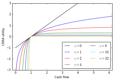
CRRA utility vs. cash flow for selected values of γ
You can look at 1 as a reference cash flow with a utility of 0. As you get more cash flow above 1, your utility goes up less and less. As you get less cash flow below 1, your utility goes down more and more. As γ goes up, this convexity effect increases. (But recall that levels don’t change choices with CRRA and same can be said for any point on the curve. Trust us, or try it in Excel!)
The key points are:
- We use a CRRA utility function to convert risky or variable cash flows to a utility, based on γ the risk aversion parameter.
- After summing utilities, we convert utility back to cash flows using the inverse function.
- This gives the certainty equivalent value of the cash flows, which discounts the cash flows based on their distribution.
- γ = 0 means you’re risk neutral. There is no discount, however variable or uncertain the cash flows. The CE value equals the sum of the cash flows.
- γ = 8 means you’re fairly risk averse. There is a large discount.
- The higher the variability of the cash flows, the greater the discount. And the higher the γ parameter, the greater the discount.
- The discount is the same, if you multiply all the cash flows by 2, or 1000, or 0.01, or x. Your risk aversion is the same at all levels of income. That property accounts for the somewhat complex formula, but it describes a risk aversion that behaves in a relatively simple way.
If we think that, to a reasonable approximation, humans are risk averse, they make consistent choices about risky outcomes, and their risk aversion is scale invariant over the range of outcomes we are studying, CE cash flow using a CRRA utility function seems like a reasonable thing to try to maximize.
In our example, we maximize certainty-equivalent cash flow for a retiree over 30 years of retirement, over the historical distribution of outcomes for the 59 30-year retirement cohorts 1928-1986. The retiree’s risk aversion parameter is 8. This is risk-averse (but not extremely so).
Maximizing CE spending means the retiree plans to spend down the entire portfolio after 30 years. Presumably the retiree knows how long he or she will need retirement income. Perhaps the retiree is 75 and 30 seems like a reasonable maximum to plan for, perhaps the retiree has an alternative to hedge longevity risk, like an insurance plan or tontine.
3. How does this work in TensorFlow?
TensorFlow is like a spreadsheet. You start with a set of constants and variables. You create a calculation that uses operations to build on the constants and variables, just like a spreadsheet. The calculation operations you define are represented by a computation graph which tracks which operations depend on which. You can tell TensorFlow to calculate any value you defined, and it will only recompute the minimum necessary operations to supply the answer. And you can program TensorFlow to optimize a function, i.e. find the variables that result in the best value for an operation.
We want to set the values for these 3 variables, in order to maximize CE cash flow:
1: Constant spending (a single value): A constant inflation-adjusted amount you withdraw each year in retirement. This is like the 4% in Bengen’s 4% rule. The inflation-adjusted value of this annual withdrawal never changes.
2: Variable spending (30 values, one for each year of retirement, i.e. a list or vector): A variable percentage of your portfolio value you withdraw each year. In contrast to the Bengen 4% rule, we’re, saying, if the portfolio appreciates, you can safely withdraw an additional amount based on the current value of the portfolio. Your total spending is the sum of 1) constant spending and 2) variable spending.
3: Stock allocation (30 values, one for each year): We are going to study a portfolio with 2 assets: S&P 500 stocks and 10-year Treasurys.3
Our key constants are:
- γ = 8. (a constant because we are not optimizing its value, unlike the variables above).
- A portfolio starting value: 100.
- Inflation-adjusted stock returns 1928-2015 (all numbers we use are inflation-adjusted, and we maximize inflation-adjusted cash flow).
- Inflation-adjusted bond returns 1928-2015.
Operations:
- Calculate 59 30-vectors, each one representing the cash flow of one 30-year retirement cohort 1928-1986, using the given constant spending, variable spending, and stock allocation.
- Calculate the certainty equivalent cash flow of each cohort using γ.
- Calculate the certainty equivalent cash flow over all cohorts using γ.
- Tell TensorFlow to find the variables that result in the highest CE spending over all cohorts.
We initialize the variables to some reasonable first approximation.
TensorFlow calculates the gradient of the objective over all variables, and gradually adjusts each variable to find the best value.
See TensorFlow / python code on GitHub.
Below, you can click to set the value of γ and see how the solution and outcome evolves.
| const_spend | var_spend | stocks | bonds | spend_mean | spend_min | spend_max | |
|---|---|---|---|---|---|---|---|
| 2.25168 | 2.203127 | 81.789336 | 18.210664 | 4.604840 | 3.724279 | 5.431478 | |
| 1 | 2.25168 | 2.287617 | 81.584539 | 18.415461 | 4.731527 | 3.418391 | 6.254532 |
| 2 | 2.25168 | 2.349896 | 81.042750 | 18.957250 | 4.826188 | 3.513405 | 6.347958 |
| 3 | 2.25168 | 2.400992 | 80.498949 | 19.501051 | 4.932219 | 3.517121 | 7.302567 |
| 4 | 2.25168 | 2.457950 | 79.886688 | 20.113312 | 5.049210 | 3.505759 | 7.408146 |
| 5 | 2.25168 | 2.529678 | 79.489911 | 20.510089 | 5.197089 | 3.386326 | 7.941039 |
| 6 | 2.25168 | 2.606445 | 79.154073 | 20.845927 | 5.351562 | 3.420979 | 8.891322 |
| 7 | 2.25168 | 2.713869 | 78.390047 | 21.609953 | 5.557626 | 3.522455 | 9.081053 |
| 8 | 2.25168 | 2.836364 | 77.651215 | 22.348785 | 5.743047 | 3.348000 | 9.203257 |
| 9 | 2.25168 | 2.981631 | 77.651215 | 22.348785 | 5.980422 | 3.458124 | 10.540080 |
| 10 | 2.25168 | 3.137015 | 77.086559 | 22.913441 | 6.282104 | 3.425701 | 11.225243 |
| 11 | 2.25168 | 3.303466 | 76.476785 | 23.523215 | 6.610572 | 3.473727 | 11.643038 |
| 12 | 2.25168 | 3.478377 | 76.048041 | 23.951959 | 6.969665 | 3.317807 | 13.439483 |
| 13 | 2.25168 | 3.625880 | 75.627575 | 24.372425 | 7.310505 | 3.343283 | 15.059415 |
| 14 | 2.25168 | 3.770352 | 75.205921 | 24.794079 | 7.616833 | 3.459124 | 16.401976 |
| 15 | 2.25168 | 3.936515 | 74.476987 | 25.523013 | 7.908735 | 3.274292 | 17.074267 |
| 16 | 2.25168 | 4.134133 | 73.971955 | 26.028045 | 8.230050 | 3.366878 | 20.061546 |
| 17 | 2.25168 | 4.377164 | 73.565393 | 26.434607 | 8.588685 | 3.435252 | 22.118598 |
| 18 | 2.25168 | 4.646451 | 72.994245 | 27.005755 | 8.918598 | 3.395044 | 21.213925 |
| 19 | 2.25168 | 4.954221 | 72.523218 | 27.476782 | 9.251004 | 3.521019 | 21.152092 |
| 20 | 2.25168 | 5.292311 | 71.995758 | 28.004242 | 9.595167 | 3.708905 | 21.061695 |
| 21 | 2.25168 | 5.753135 | 71.535585 | 28.464415 | 10.053624 | 3.599248 | 20.643662 |
| 22 | 2.25168 | 6.370145 | 71.022398 | 28.977602 | 10.585032 | 3.637109 | 22.381867 |
| 23 | 2.25168 | 7.174056 | 70.527878 | 29.472122 | 11.207199 | 3.846862 | 23.833581 |
| 24 | 2.25168 | 8.313613 | 69.984383 | 30.015617 | 11.968715 | 3.682980 | 27.458563 |
| 25 | 2.25168 | 9.946128 | 69.518839 | 30.481161 | 12.956893 | 3.900901 | 29.879319 |
| 26 | 2.25168 | 12.422349 | 68.999420 | 31.000580 | 14.327986 | 3.908337 | 30.120498 |
| 27 | 2.25168 | 16.581733 | 68.496478 | 31.503522 | 16.463549 | 3.948743 | 35.387707 |
| 28 | 2.25168 | 24.927346 | 68.006998 | 31.993002 | 20.297396 | 3.750516 | 46.393183 |
| 29 | 2.25168 | 100.000000 | 67.503853 | 32.496147 | 54.071078 | 2.945589 | 135.483633 |
4. Comments and caveats.
The results above are just an approximation to an optimal solution, after running the optimizer for a few hours. However, I believe that it’s close enough to be of interest and I believe that in this day and age of practically unlimited computing resources, we can likely calculate this number to an arbitrary level of precision in a tractable amount of time. (Unless I overlooked some particularly ill-behaved property of this calculation.)
Numerical optimization works by hill climbing. Start at some point; for each variable determine its gradient, i.e. how much changing the input variable changes the objective; update each variable in the direction that improves the objective; repeat until you can’t improve the objective.
It’s a little like climbing Mount Rainier, by just looking at the very local terrain and always moving uphill. It’s worth noting that if you start too far from your objective, you might climb Mt. Adams.
Similarly, in the case of optimizing CE cash flow, we might have just found a local optimum, not a global optimum. If the shape of the solution surface isn’t convex, if the slopes are flat in more than one place, we might have found one of those and not the global optimum. So this solution is not an exact solution, but finding a very good approximation of the best solution seems tractable with sufficiently smart optimization (momentum, smarter adaptive learning rate, starting from a known pretty good spot via theory or brute force).
We see that in good years, spending rises rapidly in the last few years. The algorithm naturally tries to keep some margin of error to not run out of money, and then also naturally tries to maximize spending by spending everything in the last couple of years.
As γ increases, constant spending increases, stocks decrease, and bonds increase.
It’s worth noting that we added some soft constraints: keep allocations between 0 and 100%, i.e. you can’t go short. Keep spending parameters above zero, you can’t save more now and spend more later. Also, we constrained the stock allocation to decline over time. The reason is that a worst case of running out of money has a huge impact on CE cash flow. The worst year to retire is 1966, and the most impactful year is 1974, when stocks were down > 40%. So an unconstrained solution reduces stocks in year 9 and then brings them back up. While we laud the optimizer for sidestepping this particular worst case scenario, this is probably not a generalizable way to solve the problem. We expect stock allocation to decline over time, so we added that as a constraint, and avoid whipping the stock allocation up and down.
How the optimization handles this historical artifact highlights the contrast between a historical simulation and Monte Carlo. Using a historical simulation raises the possibility that something that worked with past paths of returns may not work in all cases in the future, even if future return relationships are broadly similar. Monte Carlos let us generate an arbitrary amount of data from a model distribution, eliminating artifacts of a particular sample.
However, a Monte Carlo simulation assumes a set of statistical relationships that don’t change over time. In fact, it seems likely that the relationships over the last 59 cohorts did change over time.
- Policy regimes, i.e. the fiscal and monetary response to growth and inflation changes under constraints like the gold standard, schools of thought that dominate policy.
- Expectations regimes, whether investors expect growth and inflation, based on how they may have conditioned by their experience and education.
- Environment regimes, changes in the world as there are wars, depressions, economies become more open.
Pre-war, dividend yields had to be higher than bond yields because stocks were perceived as risky. Then it flipped. Growth was seen as predictable, companies re-invested earnings, taxes made them less inclined to distribute. Today, once again, dividends are often higher than bond yields.
For 3 decades post-war inflation surprised to the upside, for the last 3 decades it surprised to the downside.
The beauty of a historical simulation is it answers a simple question: what parameters would have worked best in the past? Monte Carlo simulations can give you a more detailed picture, if you can only believe their opinionated assumptions about a well-behaved underlying distribution.
One has to be a bit cautious with both historical simulations, which depend on the idiosyncrasies of the past, and Monte Carlos, which assume known, stable covariances. It would be wise to look at both historical simulation and Monte Carlos, do a few Monte Carlos with the range of reasonable covariance matrix estimates, use the worst case, and run historical simulations over all cohorts, and include a margin of error (especially in the current ZIRP environment which might repeat a 1966 cohort of the damned).
Another assumption in our simulation is that a certain dollar in year 30, when you may be 90, is worth the same as a dollar in year 1.
A dollar may be worth spending on different things at 60 vs. at 90, and, in later years the retiree is more likely to be dead. With respect to the mortality issue, in the same way we are computing certainty equivalent cash flow over a distribution of market outcomes, we can also compute it over a distribution of longevity outcomes. This feature is in the code, but I will leave discussion for a future blog post. The current post is more than complex enough.
Of course, this simulation doesn’t include taxes, expenses.
Finally, there are reasons to choose a less volatile portfolio that doesn’t maximize CE cash flow, if the volatility is stomach-churning in and of itself, or if it leads the retiree to re-allocate at inopportune times or otherwise change plans in a suboptimal way.
5. Conclusion.
Optimizing CE cash flow over historical data might be flawed, it might be simplistic, or it might be useful. It’s just an itch that I’ve wanted to scratch for a while. It may seem complicated, but that’s because the problem is interesting. The one takeaway should be that if you can decide what your utility/cost function is, you can find a way to maximize it using today’s computing tools and resources.
Ultimately, you have to optimize for something. If you don’t know where you want to go, you’re not going to get there. Since we have tools to optimize complex functions, perhaps the discussion should be over what to optimize for. A CRRA framework is a good possibility to start with, although I there are others as well.
This is not investment advice! This is a historical study/mad science experiment. It may not be applicable to you, it is a work in progress, and it may contain errors.
Notes
On 9/25 I updated this post. After running for many additional hours from additional starting points, found a &gamma=8; plan that improved the original by about 1%. The change is small. But it’s important to note that the optimization doesn’t converge on a single solution quickly, and the solution varies a bit depending on the starting point. It appears more work is needed to make this analysis an aide to practical decision-making. Also added the visualization allowing you to click to see how spending plans change as γ changes.
1 TensorFlow lets you definite a calculation sort of like a spreadsheet does, and then run it on on your Nvidia GPU (Graphical Processing Unit). Modern GPUs have more transistors than CPUs, and are optimized to do many parallel floating point calculations. The way you numerically optimize a function is by calculating a gradient vs. each input, and gradually changing the inputs until you find the ones that produce the best output. 100 inputs = 100 gradients that you calculate each step, and GPUs can calculate all 100 simultaneously, and accelerate these calculations quite dramatically. That being said, this optimization seems to run 4-5x faster on CPU than GPU. ¯_(ツ)_/¯ Without knowing a lot of TensorFlow internals, a single operation that needs to be done on CPU might mean the overhead of moving data back and forth kills the GPU advantage. Or maybe the Amazon g2 GPU instances have some driver issues with TensorFlow. Them’s the breaks in numerical computing.
2 This may beg the question of lotteries, why people gamble, whether homo economicus is a realistic assumption. We’re assuming rational people here. In general in financial markets, the more risky an investment is, the higher expected return it needs to offer to find a buyer. So the assumption people prefer less risky and variable retirement cash flows seems well established. It would also be possible in theory to do the same optimization for any utility function, although some would be more troublesome than others. If we have a cost function that measures the result of a spending plan, we measure how it performs and compare spending plans. If we don’t have such a cost function, we can try different ways of constructing plans and compute the results, but we don’t have a systematic way to compare them.
3 Bengen used intermediate corporates as a bond proxy. They have a higher return than Treasurys. I would use the same data, but it would involve a trip to the library or possibly a Bloomberg. I used this easily available data. At some point I can run an update so it is comparable to Bengen’s result.