Beyond Grid Search: Using Hyperopt, Optuna, and Ray Tune to hypercharge hyperparameter tuning for XGBoost and LightGBM
Bayesian optimization of machine learning model hyperparameters works faster and better than grid search. Here’s how we can speed up hyperparameter tuning using 1) Bayesian optimization with Hyperopt and Optuna, running on… 2) the Ray distributed machine learning framework, with a unified API to many hyperparameter search algos and early stopping schedulers, and… 3) a distributed cluster of cloud instances for even faster tuning.
Outline:
- Results
- Hyperparameter tuning overview
- Bayesian optimization
- Early stopping
- Implementation details
- Baseline linear regression
- ElasticNetCV (Linear regression with L1 and L2 regularization)
- ElasticNet with GridSearchCV
- XGBoost: sequential grid search over hyperparameter subsets with early stopping
- XGBoost: Hyperopt and Optuna search algorithms
- LightGBM: Hyperopt and Optuna search algorithms
- XGBoost on a Ray cluster
- LightGBM on a Ray cluster
- Concluding remarks
1. Results
Bottom line up front: Here are results on the Ames housing data set, predicting Iowa home prices:
XGB and LightGBM using various hyperparameter optimization methodologies
| ML Algo | Search algo | CV Error (RMSE in $) |
Time h:mm::ss |
|---|---|---|---|
| XGB | Sequential Grid Search | 18302 | 1:27:14 |
| XGB | Hyperopt (1024 samples) | 18309 | 0:53:41 |
| XGB | Optuna (1024 samples) | 18325 | 0:48:02 |
| XGB | Hyperopt (2048 samples) - 32x cluster | 18030 | 1:30:58 |
| XGB | Optuna (2048 samples) - 32x cluster | 18028 | 1:29:57 |
| LightGBM | Hyperopt (1024 samples) | 18615 | 1:13:40 |
| LightGBM | Optuna (1024 samples) | 18614 | 1:08:40 |
| LightGBM | Hyperopt (2048 samples) - 32x cluster | 18459 | 1:05:19 |
| LightGBM | Optuna (2048 samples) - 32x cluster | 18458 | 0:48:16 |
Baseline linear models
| ML Algo | Search algo | CV Error (RMSE in $) | Time mm::ss |
|---|---|---|---|
| Linear Regression | – | 18192 | 0:01 |
| ElasticNet | ElasticNetCV (Grid Search) | 17964 | 0:02 |
| ElasticNet | GridSearchCV | 17964 | 0:05 |
Times for single-instance are on a local desktop with 12 threads, comparable to EC2 4xlarge. Times for cluster are on m5.large x 32 (1 head node + 31 workers).
- We saw a big speedup when using Hyperopt and Optuna locally, compared to grid search. The sequential search performed about 261 trials, so the XGB/Optuna search performed about 3x as many trials in half the time and got a similar RMSE.
- The cluster of 32 instances (64 threads) gave a modest RMSE improvement vs. the local desktop with 12 threads. I attempted to set this up so we would get some improvement in RMSE vs. local Hyperopt/Optuna (which we did with 2048 trials), and some speedup in training time (which we did not get with 64 threads). It ran twice the number of trials in slightly less than twice the time. The comparison is imperfect, local desktop vs. AWS, running Ray 1.0 on local and 1.1 on the cluster, different number of trials (better hyperparameter configs don’t get early-stopped and take longer to train). But the point was to see what kind of improvement one might obtain in practice, leveraging a cluster vs. a local desktop or laptop. Bottom line, modest benefit here from a 32-node cluster.
- RMSEs are similar across the board. XGB with 2048 trials is best by a small margin among the boosting models.
- LightGBM doesn’t offer improvement over XGBoost here in RMSE or run time. In my experience LightGBM is often faster so you can train and tune more in a given time. But we don’t see that here. Possibly XGB interacts better with ASHA early stopping.
- Similar RMSE between Hyperopt and Optuna. Optuna is consistently faster (up to 35% with LGBM/cluster).
Our simple ElasticNet baseline yields slightly better results than boosting, in seconds. This may be because our feature engineering was intensive and designed to fit the linear model. Not shown, SVR and KernelRidge outperform ElasticNet, and an ensemble improves over all individual algos.
Full notebooks are on GitHub.
2. Hyperparameter Tuning Overview
(If you are not a data scientist ninja, here is some context. If you are, you can safely skip to Bayesian optimization and implementations below.)
Any sufficiently advanced machine learning model is indistinguishable from magic, and any sufficiently advanced machine learning model needs good tuning.
Suppose you have a neural network to predict whether a stock will go up or down next week (binary classification). Suppose the neural network is described by 3 discrete hyperparameters: how many layers, how many units in each layer, and an activation function (relu or logistic). The hyperparameter optimization problem is to find the parameter vector that yields the best results.
One dumb way is an exhaustive grid search over all possible values. Another way is a random search, drawing hyperparameter values from independent uniform distributions. A smarter Bayesian search starts off sampling from independent uniform distributions but tries to learn the best region and distribution to sample from. So it works faster and better. That’s pretty much it.
To dive in a little, here is a typical modeling workflow:
- Exploratory data analysis: understand your data.
- Feature engineering and feature selection: clean, transform and engineer the best possible features
- Modeling: model selection and hyperparameter tuning to identify the best model architecture, and ensembling to combine multiple models
- Evaluation: Describe the out-of-sample error and its expected distribution.
To minimize the out-of-sample error, you minimize the error from bias, meaning the model is too simple or insufficiently sensitive to the signal in the data, and variance, meaning the model is too complex or too sensitive to noise in the training data in ways that don’t generalize out-of-sample. Modeling is 90% data prep, the other half is all finding the optimal bias-variance tradeoff.
Hyperparameters help you tune the bias-variance tradeoff. For a simple logistic regression predicting survival on the Titanic, a regularization parameter lets you control overfitting by penalizing sensitivity to any individual feature. For a massive neural network doing machine translation, the number and types of layers, units, activation function, in addition to regularization, are hyperparameters. We select the best hyperparameters using k-fold cross-validation; this is what we call hyperparameter tuning.
The regression algorithms we use in this post are XGBoost and LightGBM, which are variations on gradient boosting. Gradient boosting is an ensembling method that usually involves decision trees. A decision tree constructs rules like, if the passenger is in first class and female, they probably survived the sinking of the Titanic. Trees are powerful, but a single deep decision tree with all your features will tend to overfit the training data. A random forest algorithm builds many decision trees based on random subsets of observations and features which then vote (bagging). The outcome of a vote by weak learners is less overfitted than training on all the data rows and all the feature columns to generate a single strong learner, and performs better out-of-sample. Random forest hyperparameters include the number of trees, tree depth, and how many features and observations each tree should use.
Instead of aggregating many independent learners working in parallel, i.e. bagging, boosting uses many learners in series:
- Start with a simple estimate like the median or base rate.
- Fit a tree to the error in this prediction.
- If you can predict the error, you can adjust for it and improve the prediction. Adjust the prediction not all the way to the tree prediction, but part of the way based on a learning rate (a hyperparameter).
- Fit another tree to the error in the updated prediction and adjust the prediction further based on the learning rate.
- Iteratively continue reducing the error for a specified number of boosting rounds (another hyperparameter).
- The final estimate is the initial prediction plus the sum of all the predicted necessary adjustments (weighted by the learning rate).
The learning rate performs a similar function to voting in random forest, in the sense that no single decision tree determines too much of the final estimate. This ‘wisdom of crowds’ approach helps prevent overfitting.
Gradient boosting is the current state of the art for regression and classification on traditional structured tabular data (in contrast to less structured data like image/video/natural language processing, where deep learning, i.e. deep neural nets are state of the art).
Gradient boosting algorithms like XGBoost, LightGBM, and CatBoost have a very large number of hyperparameters, and tuning is an important part of using them.
These are the principal approaches to hyperparameter tuning:
-
Grid search: Given a finite set of discrete values for each hyperparameter, exhaustively cross-validate all combinations.
-
Random search: Given a discrete or continuous distribution for each hyperparameter, randomly sample from the joint distribution. Generally more efficient than exhaustive grid search.
-
Bayesian optimization: Sample like random search, but update the search space you sample from as you go, based on outcomes of prior searches.
-
Gradient-based optimization: Attempt to estimate the gradient of the cross-validation metric with respect to the hyperparameters and ascend/descend the gradient.
-
Evolutionary optimization: Sample the search space, discard combinations with poor metrics, and genetically evolve new combinations based on the successful combinations.
-
Population-based training: A method of performing hyperparameter optimization at the same time as training.
In this post, we focus on Bayesian optimization with Hyperopt and Optuna.
3. Bayesian Optimization
What is Bayesian optimization? When we perform a grid search, the search space is a prior: we believe that the best hyperparameter vector is in this search space. And a priori each hyperparameter combination has equal probability of being the best combination (a uniform distribution). So we try them all and pick the best one.
Perhaps we might do two passes of grid search. After an initial search on a broad, coarsely spaced grid, we do a deeper dive in a smaller area around the best metric from the first pass, with a more finely-spaced grid. In Bayesian terminology, we updated our prior.
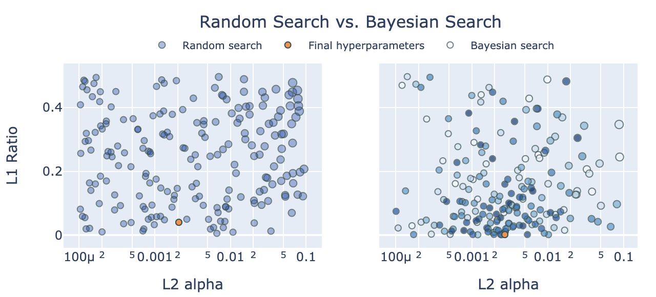
Bayesian optimization starts by sampling randomly, e.g. 30 combinations, and computes the cross-validation metric for each of the 30 randomly sampled combinations using k-fold cross-validation. Then the algorithm updates the distribution it samples from, so that it is more likely to sample combinations similar to the good metrics, and less likely to sample combinations similar to the poor metrics. As it continues to sample, it continues to update the search distribution it samples from, based on the metrics it finds.
(The size of the markers corresponds to the size of RMSE. On the left, markers are the same color, but if two markers overlap the alpha will show darker overlap. On the right marker color corresponds ot the search order, so we can see later trials are close to the final value. Hover the mouse over markers for more info.)
If good metrics are not uniformly distributed, but found close to one another in a Gaussian distribution or any distribution which we can model, then Bayesian optimization can exploit the underlying pattern, and is likely to be more efficient than grid search or naive random search.
HyperOpt is a Bayesian optimization algorithm by James Bergstra et al., see this excellent blog post by Subir Mansukhani.
Optuna is a Bayesian optimization algorithm by Takuya Akiba et al., see this excellent blog post by Crissman Loomis.
4. Early Stopping
If, while evaluating a hyperparameter combination, the evaluation metric is not improving in training, or not improving fast enough to beat our best to date, we can discard a combination before fully training on it. Early stopping of unsuccessful training runs increases the speed and effectiveness of our search.
XGBoost and LightGBM helpfully provide early stopping callbacks to check on training progress and stop a training trial early (XGBoost ; LightGBM). Hyperopt, Optuna, and Ray use these callbacks to stop bad trials quickly and accelerate performance.
In this post, we will use the Asynchronous Successive Halving Algorithm (ASHA) for early stopping, described in this blog post.
Further reading:
- Hyper-Parameter Optimization: A Review of Algorithms and Applications Tong Yu, Hong Zhu (2020)
- Hyperparameter Search in Machine Learning, Marc Claesen, Bart De Moor (2015)
- Hyperparameter Optimization, Matthias Feurer, Frank Hutter (2019)
5. Implementation Details
We use data from the Ames Housing Dataset. The original data set has 79 raw features. The data we will use has 100 features with a fair amount of feature engineering from my own attempt at modeling, which was in the top 5% or so when I submitted it to Kaggle. We model the log of the sale price, and use RMSE as our metric for model selection. We convert the RMSE back to raw dollar units for easier interpretability.
We use 4 regression algorithms:
- LinearRegression: baseline with no hyperparameters
- ElasticNet: Linear regression with L1 and L2 regularization (2 hyperparameters).
- XGBoost
- LightGBM
We use 5 approaches:
- Native CV: In sklearn if an algorithm xxx has hyperparameters it will often have an xxxCV version, like ElasticNetCV, which performs automated grid search over hyperparameter iterators with specified kfolds.
- GridSearchCV: Abstract grid search that can wrap around any sklearn algorithm, running multithreaded trials over specified kfolds.
- Manual sequential grid search: How we typically implement grid search with XGBoost, which doesn’t play very well with GridSearchCV and has too many hyperparameters to tune in one pass.
- Ray on local desktop: Hyperopt and Optuna with ASHA early stopping.
- Ray on AWS cluster: Additionally scale out to run a single hyperparameter optimization task over many instances in a cluster.
6. Baseline linear regression
- Use the same kfolds for each run so the variation in the RMSE metric is not due to variation in kfolds.
- We fit on the log response, so we convert error back to dollar units, for interpretability.
sklearn.model_selection.cross_val_scorefor evaluation- Jupyter
%%timemagic for wall time n_jobs=-1to run folds in parallel using all CPU cores available.- Note the wall time < 1 second and RMSE of 18192.
- Full notebooks are on GitHub.
%%time

# always use same RANDOM_STATE k-folds for comparability between tests, reproducibility
RANDOMSTATE = 42
np.random.seed(RANDOMSTATE)

kfolds = KFold(n_splits=10, shuffle=True, random_state=RANDOMSTATE)

MEAN_RESPONSE=df[response].mean()
def cv_to_raw(cv_val, mean_response=MEAN_RESPONSE):
    """convert log1p rmse to underlying SalePrice error"""
    # MEAN_RESPONSE assumes folds have same mean response, which is true in expectation but not in each fold
    # we can also pass the mean response for each fold
    # but we're really just looking to consistently convert the log value to a more meaningful unit
    return np.expm1(mean_response+cv_val) - np.expm1(mean_response)

lr = LinearRegression()
# compute CV metric for each fold
scores = -cross_val_score(lr, df[predictors], df[response],
                          scoring="neg_root_mean_squared_error",
                          cv=kfolds,
                          n_jobs=-1)
raw_scores = [cv_to_raw(x) for x in scores]
print("Raw CV RMSE %.0f (STD %.0f)" % (np.mean(raw_scores), np.std(raw_scores)))
Raw CV RMSE 18192 (STD 1839)
Wall time: 65.4 ms
7. ElasticNetCV
- ElasticNet is linear regression with L1 and L2 regularization (2 hyperparameters).
- When we use regularization, we need to scale our data so that the coefficient penalty has a similar impact across features. We use a pipeline with RobustScaler for scaling.
- Fit a model and extract hyperparameters from the fitted model.
- Then we do
cross_val_scorewith reported hyperparams (There doesn’t appear to be a way to extract the score from the fitted model without refitting) - Verbose output reports 130 tasks, for full grid search on 10 folds we would expect 13x9x10=1170. Apparently a clever optimization.
- Note the modest reduction in RMSE vs. linear regression without regularization.
elasticnetcv = make_pipeline(RobustScaler(),
                             ElasticNetCV(max_iter=100000,
                                          l1_ratio=[0.01, 0.05, 0.1, 0.2, 0.3, 0.4, 0.5, 0.6, 0.7, 0.8, 0.9, 0.95, 0.99],
                                          alphas=np.logspace(-4, -2, 9),
                                          cv=kfolds,
                                          n_jobs=-1,
                                          verbose=1,
                                         ))

#train and get hyperparams
elasticnetcv.fit(df[predictors], df[response])
l1_ratio = elasticnetcv._final_estimator.l1_ratio_
alpha = elasticnetcv._final_estimator.alpha_
print('l1_ratio', l1_ratio)
print('alpha', alpha)

# evaluate using kfolds on full dataset
# I don't see API to get CV error from elasticnetcv, so we use cross_val_score
elasticnet = ElasticNet(alpha=alpha,
                        l1_ratio=l1_ratio,
                        max_iter=10000)

scores = -cross_val_score(elasticnet, df[predictors], df[response],
                          scoring="neg_root_mean_squared_error",
                          cv=kfolds,
                          n_jobs=-1)
raw_scores = [cv_to_raw(x) for x in scores]
print()
print("Log1p CV RMSE %.04f (STD %.04f)" % (np.mean(scores), np.std(scores)))
print("Raw CV RMSE %.0f (STD %.0f)" % (np.mean(raw_scores), np.std(raw_scores)))
l1_ratio 0.01
alpha 0.0031622776601683794

Log1p CV RMSE 0.1030 (STD 0.0109)
Raw CV RMSE 18061 (STD 2008)
CPU times: user 5.93 s, sys: 3.67 s, total: 9.6 s
Wall time: 1.61 s
8. GridSearchCV
- Identical result, runs a little slower.
- GridSearchCV verbose output shows 1170 jobs, which is the expected number 13x9x10.
gs = make_pipeline(RobustScaler(),
                   GridSearchCV(ElasticNet(max_iter=100000),
                                param_grid={'l1_ratio': [0.01, 0.05, 0.1, 0.2, 0.3, 0.4, 0.5, 0.6, 0.7, 0.8, 0.9, 0.95, 0.99],
                                            'alpha': np.logspace(-4, -2, 9),
                                           },
                                scoring='neg_root_mean_squared_error',
                                refit=True,
                                cv=kfolds,
                                n_jobs=-1,
                                verbose=1
                               ))

# do cv using kfolds on full dataset
gs.fit(df[predictors], df[response])
print('best params', gs._final_estimator.best_params_)
print('best score', -gs._final_estimator.best_score_)
l1_ratio = gs._final_estimator.best_params_['l1_ratio']
alpha = gs._final_estimator.best_params_['alpha']

# eval similarly to before
elasticnet = ElasticNet(alpha=alpha,
                        l1_ratio=l1_ratio,
                        max_iter=100000)
print(elasticnet)

scores = -cross_val_score(elasticnet, df[predictors], df[response],
                          scoring="neg_root_mean_squared_error",
                          cv=kfolds,
                          n_jobs=-1)
raw_scores = [cv_to_raw(x) for x in scores]
print()
print("Log1p CV RMSE %.06f (STD %.04f)" % (np.mean(scores), np.std(scores)))
print("Raw CV RMSE %.0f (STD %.0f)" % (np.mean(raw_scores), np.std(raw_scores)))
best params {'alpha': 0.0031622776601683794, 'l1_ratio': 0.01}
best score 0.10247177583755482
ElasticNet(alpha=0.0031622776601683794, l1_ratio=0.01, max_iter=100000)

Log1p CV RMSE 0.103003 (STD 0.0109)
Raw CV RMSE 18061 (STD 2008)

Wall time: 5 s
9. XGBoost with sequential grid search
It should be possible to use GridSearchCV with XGBoost. But when we also try to use early stopping, XGBoost wants an eval set. OK, we can give it a static eval set held out from GridSearchCV. Now, GridSearchCV does k-fold cross-validation in the training set but XGBoost uses a separate dedicated eval set for early stopping. It seems like a bit of a Frankenstein methodology. See the notebook for the attempt at GridSearchCV with XGBoost and early stopping if you’re really interested.
Instead we write our own grid search that gives XGBoost the correct hold-out set for each CV fold:
EARLY_STOPPING_ROUNDS=100  # stop if no improvement after 100 rounds

def my_cv(df, predictors, response, kfolds, regressor, verbose=False):
    """Roll our own CV
    train each kfold with early stopping
    return average metric, sd over kfolds, average best round"""
    metrics = []
    best_iterations = []

    for train_fold, cv_fold in kfolds.split(df):
        fold_X_train=df[predictors].values[train_fold]
        fold_y_train=df[response].values[train_fold]
        fold_X_test=df[predictors].values[cv_fold]
        fold_y_test=df[response].values[cv_fold]
        regressor.fit(fold_X_train, fold_y_train,
                      early_stopping_rounds=EARLY_STOPPING_ROUNDS,
                      eval_set=[(fold_X_test, fold_y_test)],
                      eval_metric='rmse',
                      verbose=verbose
                     )
        y_pred_test=regressor.predict(fold_X_test)
        metrics.append(np.sqrt(mean_squared_error(fold_y_test, y_pred_test)))
        best_iterations.append(regressor.best_iteration)
    return np.average(metrics), np.std(metrics), np.average(best_iterations)
XGBoost has many tuning parameters so an exhaustive grid search has an unreasonable number of combinations. Instead, we tune reduced sets sequentially using grid search and use early stopping.
This is the typical grid search methodology to tune XGBoost:
XGBoost tuning methodology
- Set an initial set of starting parameters.
- Tune sequentially on groups of hyperparameters that don’t interact too much between groups, to reduce the number of combinations tested.
- First, tune
max_depth. - Then tune
subsample,colsample_bytree, andcolsample_bylevel. - Finally, tune
learning rate: a lower learning rate will need more boosting rounds (n_estimators).
- First, tune
- Do 10-fold cross-validation on each hyperparameter combination. Pick hyperparameters to minimize average RMSE over kfolds.
- Use XGboost early stopping to halt training in each fold if no improvement after 100 rounds.
- After tuning and selecting the best hyperparameters, retrain and evaluate on the full dataset without early stopping, using the average boosting rounds across xval kfolds.1
- As discussed, we use the XGBoost sklearn API and roll our own grid search which understands early stopping with k-folds, instead of GridSearchCV. (An alternative would be to use native xgboost .cv which understands early stopping but doesn’t use sklearn API (uses DMatrix, not numpy array or dataframe))
- We write a helper function
cv_over_param_dictwhich takes a list ofparam_dictdictionaries, runs trials over all dictionaries, and returns the bestparam_dictdictionary plus a dataframe of results. - We run
cv_over_param_dict3 times to do 3 grid searches over our 3 tuning rounds.
BOOST_ROUNDS=50000   # we use early stopping so make this arbitrarily high

def cv_over_param_dict(df, param_dict, predictors, response, kfolds, verbose=False):
    """given a list of dictionaries of xgb params
    run my_cv on params, store result in array
    return updated param_dict, results dataframe
    """
    start_time = datetime.now()
    print("%-20s %s" % ("Start Time", start_time))

    results = []

    for i, d in enumerate(param_dict):
        xgb = XGBRegressor(
            objective='reg:squarederror',
            n_estimators=BOOST_ROUNDS,
            random_state=RANDOMSTATE,
            verbosity=1,
            n_jobs=-1,
            booster='gbtree',
            **d
        )

        metric_rmse, metric_std, best_iteration = my_cv(df, predictors, response, kfolds, xgb, verbose=False)
        results.append([metric_rmse, metric_std, best_iteration, d])

        print("%s %3d result mean: %.6f std: %.6f, iter: %.2f" % (datetime.strftime(datetime.now(), "%T"), i, metric_rmse, metric_std, best_iteration))

    end_time = datetime.now()
    print("%-20s %s" % ("Start Time", start_time))
    print("%-20s %s" % ("End Time", end_time))
    print(str(timedelta(seconds=(end_time-start_time).seconds)))

    results_df = pd.DataFrame(results, columns=['rmse', 'std', 'best_iter', 'param_dict']).sort_values('rmse')
    display(results_df.head())

    best_params = results_df.iloc[0]['param_dict']
    return best_params, results_df

# initial hyperparams
current_params = {
    'max_depth': 5,
    'colsample_bytree': 0.5,
    'colsample_bylevel': 0.5,
    'subsample': 0.5,
    'learning_rate': 0.01,
}

##################################################
# round 1: tune depth
##################################################
max_depths = list(range(2,8))
grid_search_dicts = [{'max_depth': md} for md in max_depths]
# merge into full param dicts
full_search_dicts = [{**current_params, **d} for d in grid_search_dicts]

# cv and get best params
current_params, results_df = cv_over_param_dict(df, full_search_dicts, predictors, response, kfolds)

##################################################
# round 2: tune subsample, colsample_bytree, colsample_bylevel
##################################################
# subsamples = np.linspace(0.01, 1.0, 10)
# colsample_bytrees = np.linspace(0.1, 1.0, 10)
# colsample_bylevel = np.linspace(0.1, 1.0, 10)
# narrower search
subsamples = np.linspace(0.25, 0.75, 11)
colsample_bytrees = np.linspace(0.1, 0.3, 5)
colsample_bylevel = np.linspace(0.1, 0.3, 5)
# subsamples = np.linspace(0.4, 0.9, 11)
# colsample_bytrees = np.linspace(0.05, 0.25, 5)

grid_search_dicts = [dict(zip(['subsample', 'colsample_bytree', 'colsample_bylevel'], [a, b, c]))
                     for a,b,c in product(subsamples, colsample_bytrees, colsample_bylevel)]
# merge into full param dicts
full_search_dicts = [{**current_params, **d} for d in grid_search_dicts]
# cv and get best params
current_params, results_df = cv_over_param_dict(df, full_search_dicts, predictors, response, kfolds)

# round 3: learning rate
learning_rates = np.logspace(-3, -1, 5)
grid_search_dicts = [{'learning_rate': lr} for lr in learning_rates]
# merge into full param dicts
full_search_dicts = [{**current_params, **d} for d in grid_search_dicts]

# cv and get best params
current_params, results_df = cv_over_param_dict(df, full_search_dicts, predictors, response, kfolds, verbose=False)
The total training duration (the sum of times over the 3 iterations) is 1:24:22. This time may be an underestimate, since this search space is based on prior experience.
Finally, we refit using the best hyperparameters and evaluate:
xgb = XGBRegressor(
    objective='reg:squarederror',
    n_estimators=3438,
    random_state=RANDOMSTATE,
    verbosity=1,
    n_jobs=-1,
    booster='gbtree',
    **current_params
)

print(xgb)

scores = -cross_val_score(xgb, df[predictors], df[response],
                          scoring="neg_root_mean_squared_error",
                          cv=kfolds,
                          n_jobs=-1)

raw_scores = [cv_to_raw(x) for x in scores]
print()
print("Log1p CV RMSE %.06f (STD %.04f)" % (np.mean(scores), np.std(scores)))
print("Raw CV RMSE %.0f (STD %.0f)" % (np.mean(raw_scores), np.std(raw_scores)))
The result essentially matches linear regression but is not as good as ElasticNet.
Raw CV RMSE 18193 (STD 2461)
10. XGBoost with Hyperopt, Optuna, and Ray
The steps to run a Ray tuning job with Hyperopt are:
- Set up a Ray search space as a config dict.
- Refactor the training loop into a function which takes the config dict as an argument and calls
tune.report(rmse=rmse)to optimize a metric like RMSE. - Call
ray.tunewith theconfigand anum_samplesargument which specifies how many times to sample.
Set up the Ray search space:
xgb_tune_kwargs = {
    "n_estimators": tune.loguniform(100, 10000),
    "max_depth": tune.randint(0, 5),
    "subsample": tune.quniform(0.25, 0.75, 0.01),
    "colsample_bytree": tune.quniform(0.05, 0.5, 0.01),
    "colsample_bylevel": tune.quniform(0.05, 0.5, 0.01),
    "learning_rate": tune.quniform(-3.0, -1.0, 0.5),  # powers of 10
}

xgb_tune_params = [k for k in xgb_tune_kwargs.keys() if k != 'wandb']
xgb_tune_params
Set up the training function. Note that some search algos expect all hyperparameters to be floats and some search intervals to start at 0. So we convert params as necessary.
def my_xgb(config):

    # fix these configs to match calling convention
    # search wants to pass in floats but xgb wants ints
    config['n_estimators'] = int(config['n_estimators'])   # pass float eg loguniform distribution, use int
    # hyperopt needs left to start at 0 but we want to start at 2
    config['max_depth'] = int(config['max_depth']) + 2
    config['learning_rate'] = 10 ** config['learning_rate']

    xgb = XGBRegressor(
        objective='reg:squarederror',
        n_jobs=1,
        random_state=RANDOMSTATE,
        booster='gbtree',
        scale_pos_weight=1,
        **config,
    )
    scores = -cross_val_score(xgb, df[predictors], df[response],
                                      scoring="neg_root_mean_squared_error",
                                      cv=kfolds)
    rmse = np.mean(scores)
    tune.report(rmse=rmse)

    return {"rmse": rmse}
Run Ray Tune:
algo = HyperOptSearch(random_state_seed=RANDOMSTATE)
# ASHA
scheduler = AsyncHyperBandScheduler()

analysis = tune.run(my_xgb,
                    num_samples=NUM_SAMPLES,
                    config=xgb_tune_kwargs,
                    name="hyperopt_xgb",
                    metric="rmse",
                    mode="min",
                    search_alg=algo,
                    scheduler=scheduler,
                    verbose=1,
                   )
Extract the best hyperparameters, and evaluate a model using them:
# results dataframe sorted by best metric
param_cols = ['config.' + k for k in xgb_tune_params]
analysis_results_df = analysis.results_df[['rmse', 'date', 'time_this_iter_s'] + param_cols].sort_values('rmse')

# extract top row
best_config = {z: analysis_results_df.iloc[0]['config.' + z] for z in xgb_tune_params}

xgb = XGBRegressor(
    objective='reg:squarederror',
    random_state=RANDOMSTATE,
    verbosity=1,
    n_jobs=-1,
    **best_config
)
print(xgb)

scores = -cross_val_score(xgb, df[predictors], df[response],
                          scoring="neg_root_mean_squared_error",
                          cv=kfolds)

raw_scores = [cv_to_raw(x) for x in scores]
print()
print("Log1p CV RMSE %.06f (STD %.04f)" % (np.mean(scores), np.std(scores)))
print("Raw CV RMSE %.0f (STD %.0f)" % (np.mean(raw_scores), np.std(raw_scores)))
With NUM_SAMPLES=1024 we obtain:
Raw CV RMSE 18309 (STD 2428)
We can swap out Hyperopt for Optuna as simply as:
algo = OptunaSearch()
With NUM_SAMPLES=1024 we obtain:
Raw CV RMSE 18325 (STD 2473)
11. LightGBM with Hyperopt and Optuna
We can also easily swap out XGBoost for LightGBM.
-
Update the search space using LightGBM equivalents.
lgbm_tune_kwargs = { "n_estimators": tune.loguniform(100, 10000), "max_depth": tune.randint(0, 5), 'num_leaves': tune.quniform(1, 10, 1.0), # xgb max_leaves "bagging_fraction": tune.quniform(0.5, 0.8, 0.01), # xgb subsample "feature_fraction": tune.quniform(0.05, 0.5, 0.01), # xgb colsample_bytree "learning_rate": tune.quniform(-3.0, -1.0, 0.5), } -
Update training function:
def my_lgbm(config):

    # fix these configs
    config['n_estimators'] = int(config['n_estimators'])   # pass float eg loguniform distribution, use int
    config['num_leaves'] = int(2**config['num_leaves'])
    config['learning_rate'] = 10**config['learning_rate']

    lgbm = LGBMRegressor(objective='regression',
                         max_bin=200,
                         feature_fraction_seed=7,
                         min_data_in_leaf=2,
                         verbose=-1,
                         n_jobs=1,
                         # these are specified to suppress warnings
                         colsample_bytree=None,
                         min_child_samples=None,
                         subsample=None,
                         **config,
                         )

    scores = -cross_val_score(lgbm, df[predictors], df[response],
                              scoring="neg_root_mean_squared_error",
                              cv=kfolds)
    rmse=np.mean(scores)
    tune.report(rmse=rmse)

    return {'rmse': np.mean(scores)}
and run as before, swapping my_lgbm in place of my_xgb. Results for LGBM: (NUM_SAMPLES=1024):
Raw CV RMSE 18615 (STD 2356)
Swapping out Hyperopt for Optuna:
Raw CV RMSE 18614 (STD 2423)
12. XGBoost on a Ray cluster
Ray is a distributed framework. We can run a Ray Tune job over many instances using a cluster with a head node and many worker nodes.
Launching Ray is straightforward. On the head node we run ray start. On each worker node we run ray start --address x.x.x.x with the address of the head node. Then in python we call ray.init() to connect to the head node. Everything else proceeds as before, and the head node runs trials using all instances in the cluster and stores results in Redis.
Where it gets more complicated is specifying all the AWS details, instance types, regions, subnets, etc.
- Clusters are defined in
ray1.1.yaml. (So far in this notebook we have been using the current production ray 1.0, but I had difficulty getting a cluster to run with ray 1.0 so I switched to the dev nightly. YMMV.) boto3and AWS CLI configured credentials are used to spawn instances, so install and configure AWS CLI- Edit
ray1.1.yamlfile with, at a minimum, your AWS region and availability zone. Imageid may vary across regions, search for the current Deep Learning AMI (Ubuntu 18.04). You may not need to specify subnet, I had an issue with an inaccessible subnet when I let Ray default the subnet, possibly bad defaults somewhere.- To obtain those variables, launch the latest Deep Learning AMI (Ubuntu 18.04) currently Version 35.0 into a small instance in your favorite region/zone
- Test that it works
- Note the 4 variables: region, availability zone, subnet, AMI imageid
- Terminate the instance and edit
ray1.1.yamlwith your region, availability zone, AMI imageid, optionally subnet - It may be advisable create your own image with all updates and requirements pre-installed and specify its AMI imageid, instead of using the generic image and installing everything at launch.
- To run the cluster:
ray up ray1.1.yaml- Creates head instance using AMI specified.
- Installs Ray and related requirements including XGBoost from
requirements.txt - Clones the druce/iowa repo from GitHub
- Launches worker nodes per auto-scaling parameters (currently we fix the number of nodes because we’re not benchmarking the time the cluster will take to auto-scale)
- After the cluster starts you can check the AWS console and note that several instances were launched.
- Check
ray monitor ray1.1.yamlfor any error messages - Run Jupyter on the cluster with port forwarding
ray exec ray1.1.yaml --port-forward=8899 'jupyter notebook --port=8899' - Open the notebook on the generated URL which is printed on the console at startup e.g. http://localhost:8899/?token=5f46d4355ae7174524ba71f30ef3f0633a20b19a204b93b4
- You can run a terminal on the head node of the cluster with
ray attach /Users/drucev/projects/iowa/ray1.1.yaml - You can ssh explicitly with the IP address and the generated private key
ssh -o IdentitiesOnly=yes -i ~/.ssh/ray-autoscaler_1_us-east-1.pem ubuntu@54.161.200.54 - Run port forwarding to the Ray dashboard with
ray dashboard ray1.1.yamland then open http://localhost:8265/ - Make sure to choose the default kernel in Jupyter to run in the correct conda environment with all installs
- Make sure to use the ray.init() command given in the startup messages.
ray.init(address='localhost:6379', _redis_password='5241590000000000') - The cluster will incur AWS charges so
ray down ray1.1.yamlwhen complete - See hyperparameter_optimization_cluster.ipynb, separated out so each notebook can be run end-to-end with/without cluster setup
- See Ray docs for additional info on Ray clusters.
Besides connecting to the cluster instead of running Ray Tune locally, no other change to code is needed to run on the cluster
analysis = tune.run(my_xgb,
                    num_samples=NUM_SAMPLES,
                    config=xgb_tune_kwargs,
                    name="hyperopt_xgb",
                    metric="rmse",
                    mode="min",
                    search_alg=algo,
                    scheduler=scheduler,
                    # add this because distributed jobs occasionally error out
                    raise_on_failed_trial=False, # otherwise no reults df returned if any trial error
                    verbose=1,
                   )
Results for XGBM on cluster (2048 samples, cluster is 32 m5.large instances):
Hyperopt (time 1:30:58)
Raw CV RMSE 18030 (STD 2356)
Optuna (time 1:29:57)
Raw CV RMSE 18028 (STD 2353)
13. LightGBM on a Ray cluster
Similarly for LightGBM:
analysis = tune.run(my_lgbm,
                    num_samples=NUM_SAMPLES,
                    config = lgbm_tune_kwargs,
                    name="hyperopt_lgbm",
                    metric="rmse",
                    mode="min",
                    search_alg=algo,
                    scheduler=scheduler,
                    raise_on_failed_trial=False, # otherwise no reults df returned if any trial error
                    verbose=1,
                   )
Results for LightGBM on cluster (2048 samples, cluster is 32 m5.large instances):
Hyperopt (time: 1:05:19) :
Raw CV RMSE 18459 (STD 2511)
Optuna (time 0:48:16):
Raw CV RMSE 18458 (STD 2511)
14. Concluding remarks
In every case I’ve applied them, Hyperopt and Optuna have obtained at least a small improvement in the best metrics I found using grid search methods. Bayesian optimization tunes faster with a less manual process vs. sequential tuning. It’s fire-and-forget.
Is Ray Tune the way to go for hyperparameter tuning? Provisionally, yes. Ray provides integration between the underlying ML (e.g. XGBoost), the Bayesian search (e.g. Hyperopt), and early stopping (ASHA). It allows us to easily swap search algorithms.
There are other alternative search algorithms in the Ray docs but these seem to be the most popular, and I haven’t got the others to run yet. If after a while I find I am always using e.g. Hyperopt and never use clusters, I might use the native Hyperopt/XGBoost integration without Ray, to access any native Hyperopt features and because it’s one less technology in the stack.
Clusters? Most of the time I don’t have a need, costs add up, did not see as large a speedup as expected. I only see ~2x speedup on the 32-instance cluster. Setting up the test I expected a bit less than 4x speedup accounting for slightly less-than-linear scaling. The longest run I have tried, with 4096 samples, ran overnight on desktop. My MacBook Pro w/16 threads and desktop with 12 threads and GPU are plenty powerful for this data set. Still, it’s useful to have the clustering option in the back pocket. In production, it may be more standard and maintainable to deploy with e.g. Terraform, Kubernetes than the Ray native YAML cluster config file. If you want to train big data at scale you need to really understand and streamline your pipeline.
It continues to surprise me that ElasticNet, i.e. regularized linear regression, performs slightly better than boosting on this dataset. I heavily engineered features so that linear methods work well. Predictors were chosen using Lasso/ElasticNet and I used log and Box-Cox transforms to force predictors to follow assumptions of least-squares. But still, boosting is supposed to be the gold standard for tabular data.
This may tend to validate one of the critiques of machine learning, that the most powerful machine learning methods don’t necessarily always converge all the way to the best solution. If you have a ground truth that is linear plus noise, a complex XGBoost or neural network algorithm should get arbitrarily close to the closed-form optimal solution, but will probably never match the optimal solution exactly. XGBoost regression is piecewise constant and the complex neural network is subject to the vagaries of stochastic gradient descent. I thought arbitrarily close meant almost indistinguishable. But clearly this is not always the case.
ElasticNet with L1 + L2 regularization plus gradient descent and hyperparameter optimization is still machine learning. It’s simply a form of ML better matched to this problem. In the real world where data sets don’t match assumptions of OLS, gradient boosting generally performs extremely well. And even on this dataset, engineered for success with the linear models, SVR and KernelRidge performed better than ElasticNet (not shown) and ensembling ElasticNet with XGBoost, LightGBM, SVR, neural networks worked best of all.
To paraphrase Casey Stengel, clever feature engineering will always outperform clever model algorithms and vice-versa2. But improving your hyperparameters will always improve your results. Bayesian optimization can be considered a best practice.
Again, the full code is on GitHub
-
It would be more sound to separately tune the stopping rounds. Just averaging the best stopping time across kfolds is questionable. In a real world scenario, we should keep a holdout test set. We should retrain on the full training dataset (not kfolds) with early stopping to get the best number of boosting rounds. Then we should measure RMSE in the test set using all the cross-validated parameters including number of boosting rounds for the expected OOS RMSE. For the purpose of comparing tuning algorithms, comparing the CV error is OK. We are evaluating how we would make model decisions using CV and not too concerned about the generalization error. One could even argue it adds a little more noise to the comparison of hyperparameter selection. But a test set would be the correct methodology in most real-world scenarios. It wouldn’t change conclusions directionally and I’m not going to rerun everything, but if I were to start over I would do it that way. ↩
-
This is not intended to make sense. ↩