How I learned to stop worrying and love PCA: The optimal threshold for PCA dimensionality reduction
PCA is an essential data science tool which uses the SVD to break down the linear relationships in data. The Gavish-Donoho optimal truncation threshold provides a simple formula to select a good threshold for dimensionality reduction.
There is nothing insignificant in the world. It all depends on the point of view. - Goethe
Mathematics is just a collection of cheap tricks and bad jokes - Lipman Bers
I came across this excellent method for selecting an optimal rank for dimensionality reduction when applying Principal Component Analysis (PCA) and the Singular Value Decomposition (SVD).
When we apply PCA for dimensionality reduction, we have to select a number of components to use for a reduced-rank approximation. The “PCA 101” best practice is to plot the singular values in the “scree” plot and look for an “elbow” where the significance of components stops dropping off rapidly, and which captures a large fraction of the variance. If the plot were a mountain, we look for the spot where scree debris rolling down the mountain would accumulate. At that point, we think we have captured the true rank of our data, and the remaining components are mostly noise.
Here is a systematic approach:
- Perform PCA on white noise with some standard deviation \(\sigma\) and model the singular value profile of white noise.
- If you assume your real data matrix has a true rank plus white noise, you can estimate the \(\sigma\) of the noise in your data by fitting your least-significant singular values to the singular value profile of white noise.
- Using this estimate of the white noise in your data, select a threshold below which additional ranks add more noise than data, or don’t improve a regression against the PCA components.
The method is described in this paper by M. Gavish and D. L. Donoho, “The Optimal Hard Threshold for Singular Values is \(4/\sqrt {3}\).”
In the rest of the post, we’ll do a quick refresher on PCA and then apply this method in Python.
PCA Review
- In my first job as a research assistant back in the 80s, PCA came up, and I asked my distinguished boss “what’s PCA?”. He answered, “it’s a way to fit everything against everything at the same time”. PCA, or more generally the SVD from which it derives, is not just dimensionality reduction, it’s an X-ray of our data to find all the linear relationships. Starting from an SVD decomposition, you can semi-trivially implement, not only compression and dimensionality reduction, but regression, classification like facial recognition, anomaly detection, and recommender systems. For pretty much anything you want to do with data, PCA and SVD can be a good starting point.
- Geometrically, every linear algebra transformation is rotation, dilation, reflection or projection, and compositions thereof. Linear transformations can be represented as matrices. And they operate on matrices. Linear transformations are a vector space, and so is the data they operate on.1
- We can decompose or factorize any matrix in different ways. Suppose we have a data matrix with \(m\) rows (observations, samples) and \(n\) columns (features, predictors). Singular value decomposition factorizes any \(m \times n\) matrix \(A\) as: \(A = U \Sigma V^T\) where (don’t worry too much if the bullets below are Greek, just skip down to the example after the linear algebra):
- \(U\) is the \(m \times m\) orthogonal matrix of the eigenvectors of \(A^TA\), the left singular vectors. They capture all the relationships between the observation rows.
- \(V^T\) is the \(n \times n\) orthogonal matrix of the eigenvectors of \(AA^T\), the right singular vectors. They capture all the relationships between the feature columns.
- \(\Sigma\) is a \(m \times n\) diagonal dilation (scaling) matrix, the singular values. The left and right singular vector matrices are orthogonal unit vectors with norm 1, so they don’t contain any scaling data. The singular values describe the scale of each principal component, connecting the unitary scale of the singular vectors to the true scale of the original data. The singular values are, by convention, sorted by size as you go down the diagonal. Sorting makes the decomposition unique up to changes in sign. The eigenvalues are guaranteed to be real and positive because \(A^TA\) and \(AA^T\) are products of matrices by their transpose and therefore positive definite by construction.
- The existence of this decomposition proves the first sentence of this bullet: any matrix transformation can be decomposed into a combination of an orthogonal matrix rotoreflection in row space, a dilation scaling of each column by a factor (projection onto lower-dimentional subspace if a factor is 0), and an orthogonal matrix rotoreflection in column space. Alternatively, any linear transformation can be viewed as a dilation in an appropriately chosen basis, plus a rotation. Any linear transformation can be viewed as, rotate to some appropriate basis, do dilation only, rotate again.
- The principal components are defined as \(P = U\Sigma\), so by substitution we get the original data back as \(A=PV^T\). Multiplying each side by \(V\) we get \(P=AV\). (The inverse of an orthogonal matrix is its transpose.) So matrix \(V\) contains the loadings that transform original feature columns into principal components; and vice versa, \(V^T\) contains the loadings that transform principal component columns back into original feature columns. Each principal component is a weighted average of the feature columns, where the weights form an orthogonal matrix.2
- An orthogonal matrix is just a rotation (and optional reflection). PCA can be viewed as rotating \(A\) to \(P\) using \(V\) as a basis transformation to a better basis for this data set. Why is \(V^T\) a better (or the best) basis? Suppose you are analyzing a spiral galaxy. Some weird basis from a random point in random directions may not be an ideal basis. A good coordinate system might be:
- Set the origin at the center of the galaxy.
- Set the \(x\)-axis along the principal axis which maximizes the variance along the \(x\)-axis and minimizes the variance perpendicular to the \(x\)-axis (along the remaining axes).
- Set the \(y\)-axis orthogonal to the \(x\)-axis in the direction that maximizes the remaining variance.
- Set the \(z\)-axis to the only possible axis orthogonal to the first two, which is the axis capturing the least-possible variation.
- This basis transformation conserves overall variance and relationships of data (all distances and angles between data points).
- In this basis, covariances are eliminated, computation is easier, and interpretation can be more intuitive. And we can reduce dimensionality by ignoring dimensions that are mostly noise.
- Each principal component column is a linear combination of the original feature columns. You can think of each principal component as representing an independent latent variable. For instance, if I try to predict a recession using a large dataset of economic activity, I might find principal components corresponding to aggregate demand, inflation, monetary conditions, labor markets, consumer demand, investment demand, fiscal policy, and the foreign sector.
- Each principal component is independent. Each principal component feature column has 0 correlation with every other principal component feature column; the slope of a regression line between any two principal components is 0.
- The labor market principal component might have big loadings on employment growth and wages, big negative loadings on the unemployment rate and jobless claims, and then it must add and subtract enough of the other features to eliminate any correlation with any other principal component. The labor principal component’s singular value would measure its contribution to the variance.
- We can say that the SVD decomposes \(A\) into a rotation in column space \(U\), a rotation in row space \(V^T\), and a diagonal dilation matrix \(\Sigma\). Remember what we said: a matrix represents data or a linear transformation on data. Our \(m \times n\) data matrix could be viewed as a transformation matrix we can apply to any \(n \times k\) matrix, and it will rotate each column of the matrix in \(A\)’s row space, scale it and rotate the result in column space to give a \(m \times k\) matrix. We aren’t necessarily interested in how our data acts as a transformation. A more useful way of looking at the SVD is, it decomposes the data into principal component rows \(P\) rotated by \(V^T\), or principal component columns \(\Sigma V^T\) rotated by \(U\).3
A PCA Example
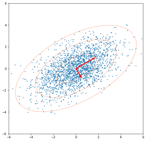
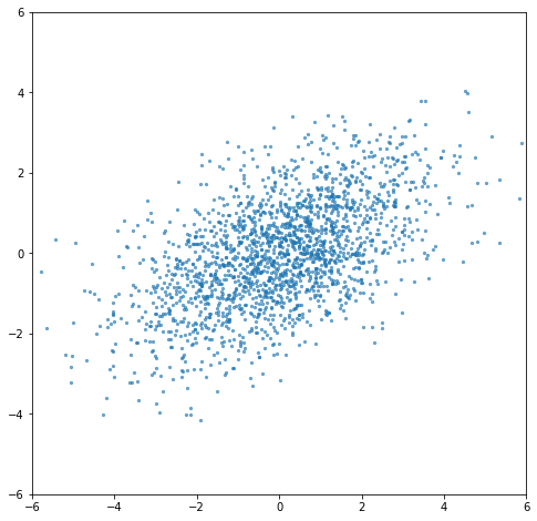
Suppose we generate some random 2-dimensional data, with standard deviation 2 in the \(x\) direction and 1 in the \(y\) direction. Then we rotate it 30° counterclockwise. Now the data columns are correlated, each point is a mix of the original \(x\) and \(y\) directions.
Now we perform the SVD on our data. If we multiply our right singular vectors (norm=1) by the singular values, we get vectors showing our principal axes, with their norms being the standard deviations we used to construct the data.
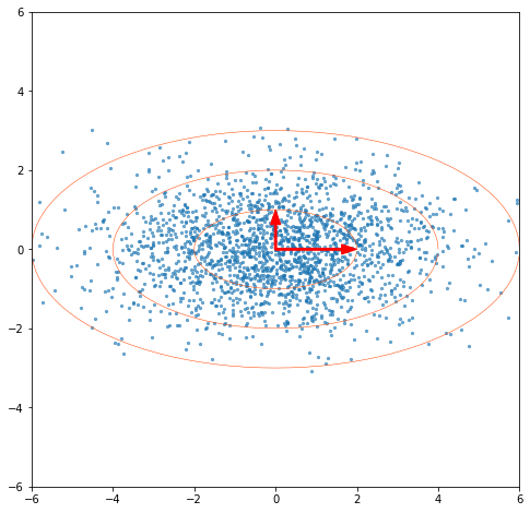
If we multiply our left singular vectors by the singular values, we get our principal components. In this example we have our random unrotated data back. The PCA rotation unf**ks the basis or finds the best basis for the data in the sense of minimizing variance in the coordinates and zeroing their covariances, whether it’s in 2 or higher dimensions.
“I regressed everything with this one cheap trick”
Rotating the basis properly turns out to be the better part of regression. Suppose I take figure 5 and use the principal axis eigenvectors as my basis. In this coordinate system, the standard deviation ellipses become circles. Now, suppose I know some \(x\) value and I want to predict \(y\). The points with a known \(x\) form a line (generally not vertical in this basis). If I project the origin onto that line, I get the point closest to the origin in likelihood space and therefore, after I convert that point to coordinates in the original basis, I get the maximum-likelihood estimate of \(y\). So, not only does the SVD provide a simple regression formula, it breaks down the data in such a way, that if I have \(n\) known variables, I can project the origin onto the subspace defined by those \(n\) variables, and get the maximum-likelihood estimate of the missing variables. That’s what ‘regressing everything against everything’ means. Any regression you might want to do falls out of the SVD via matrix multiplication.
It’s worth mentioning one interesting minor mathematical difference between PCA and ordinary least squares regression. When we do standard OLS regression with \(x\) as the explanatory variable and \(y\) as the dependent variable, we get a regression line defined by \(y=ax +b\). We estimate the \(a\) and \(b\) that minimize the squared error in the \(y\) direction. If we then fit \(x = cy +d\) on the same training data, \(c\) will not be exactly \(1/a\), because we are minimizing the error in the \(x\) direction. Even if you have a perfect normal distribution, you only get the same regression line if that slope is 1. There will also be a difference depending on the departure from normality, outliers etc. In other words, vanilla OLS linear regression minimizes the expected squared vertical distance between the regression line and target variable. When you flip the axes, you are minimizing what was formerly the horizontal distance. PCA fits everything against everything simultaneously, and solves for principal axes which minimize the square of the error as measured by the distance between points and the principal axes via perpendicular projection, instead of horizontally or vertically depending on the target. (The ‘vanilla’ \(x\) v. \(y\) regression can also fall out of an SVD via the pseudoinverse.)
Optimal PCA truncation
To recap, when we apply SVD, we rotate our data into a basis aligned with the principal component vectors, or express the data in terms of independent principal components or latent variables, which are linear combinations of the original features. This gives insight into the true rank or dimensionality of our data. For instance, if the true rank of the data is 2, because the other features are linear combinations of the first 2 (modulo noise), we can compress the data in an \(m \times n\) matrix down to \(m \times 2\) without loss of information. We can apply machine learning on a smaller \(m \times 2\) matrix which may be faster and yield better results without the noise.
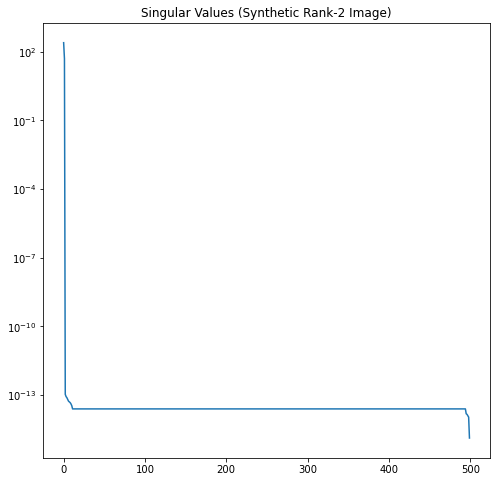
Let’s generate an image with a true rank of 2. To do this, we initially create \(U\) and \(V\) as \(500 \times 2\) matrices.
For U, we choose these 2 principal components (we just want something with interesting variation to make a good test image):
\[U_1 = cos(5x) * e^{-x^2}\] \[U_2 = sin(7x)\]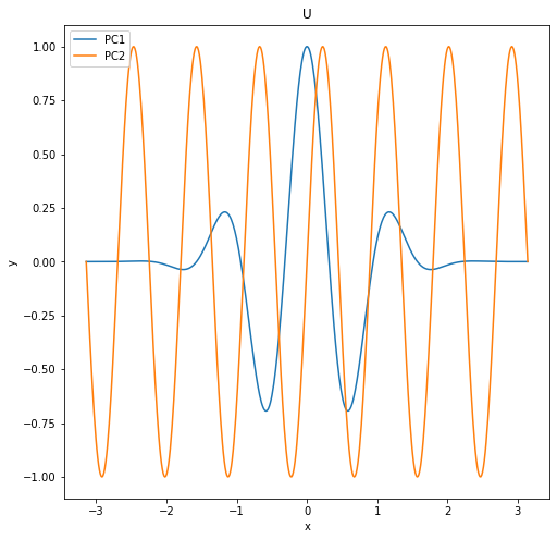
For V, we choose these 2 principal components:
\[V_1 = sin(11x) e^{-x^2}\] \[V_2 = cos(13x)\]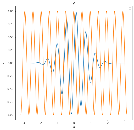
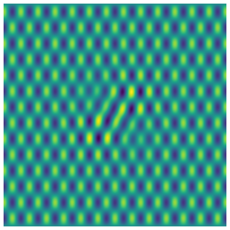
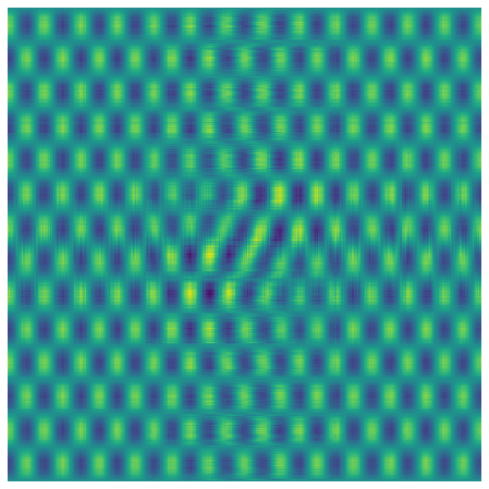
and make a \(\Sigma\) equal to the identity matrix and compute a \(500 \times 500\) pixel image as \(U\Sigma V^T\)
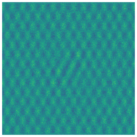
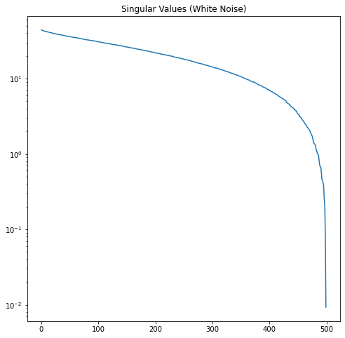
Now let’s create some white noise with \(\sigma=1\) and add it to the image:
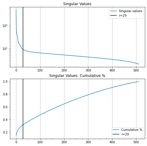
Now let’s look at the singular value profiles for the original image, the white noise, and the combined noisy image.
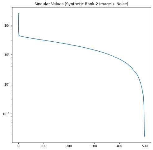
In Figure 12, it’s easy to see where the rank-2 singular values of our noisy image run out of significance and the noise starts to dominate.
In this example, we know the \(\sigma\) of our noise and number of rows \(m\). According to the Gavish-Donoho paper, the truncation threshold for a square matrix can be computed as \(\frac{4}{\sqrt{3}}\sqrt m \sigma\). Here this is approximately 51.6. We select all the singular values larger than the threshold. This correctly truncates the rank to 2.
(In other words, we take our original SVD \(A=U \Sigma V^T\) and we keep only the first 2 columns of \(U\), the top left 2x2 part of \(\Sigma\), and the first 2 rows of \(V^T\). We then recompute the reduced-rank approximation of \(A\) from the truncated SVD matrices of the noisy image as \(A_2=U_2 \Sigma_2 V_2^T\).)
We are still transforming our 500x500 matrix \(\in\mathbb{R}^{500\times 500}\) into another 500x500 matrix, but we are projecting it onto a lower-dimensional rank-2 (plane) subspace of \(\mathbb{R}^{500\times 500}\).
We can see that this does a good job of reconstituting our matrix and eliminating most of the noise.
Usually, we don’t know the \(\sigma\) of the noise. Gavish-Donoho gives us a way to estimate the optimal hard threshold \(\hat{\tau}_*\) based on the median singular value \(y_{med}\) and the aspect ratio \(\beta=m/n\) of the matrix (equations 4 and 5 of the paper). Estimate the optimal hard threshold coefficient \(\omega(\beta)\) as
\[\displaystyle \omega(\beta) \approx 0.56 \beta^3 - 0.95 \beta^2 + 1.82 \beta + 1.43\]The singular value hard threshold is then
\[\displaystyle \hat{\tau}_* = \omega(\beta) y_{med}\]This formula says principal components with singular values less than \(\hat{\tau}_*\) will add more noise than signal to an estimated low-rank matrix. When we apply these formulas we get almost the identical threshold (51.8 vs. 51.6) and the identical rank-2 approximation.
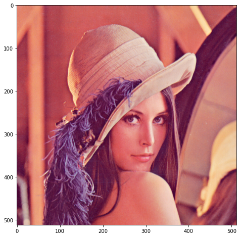
Finally, let’s apply the same process to a photo, instead of a contrived test image:
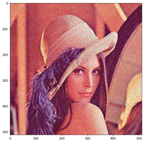
We add a small amount of noise:
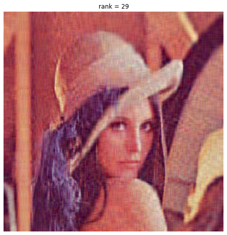
We compute our optimal PCA truncation rank as 29, which yields this image:
We compare our ‘optimally-truncated’ image to a rank-100 image:
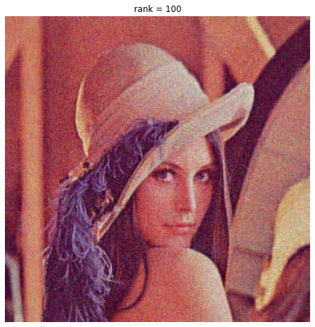
The rank-29 compression is OK quality, and 29 is close to what we get by eyeballing the elbow in the singular values. But it doesn’t perform noise reduction. Adding more dimensions does improve the image, we get more photographic detail, which so the additional dimensions aren’t perfect white noise.
One possible problem with the Gavish-Donoho threshold is that it’s trying to minimize the MSE between a target matrix and the truncated representation, assuming the target is a low rank matrix plus noise. But true optimal truncation depends on what we are going to use low-rank output for, and what our loss function is. Sometimes the low-rank vectors look like white noise but contain information we need to process downstream. If we’re trying to read an inscription on a ring in this photo, we might be better off with full-rank data. The Goethe quote up top seems on point, it’s all a matter of perspective.
Nevertheless, the Gavish-Donoho rank is a good starting point and seems to capture the essential information of this photo for downstream processing, like facial recognition or image classification. One can always add additional ranks for a margin of safety. Or cross-validate the number of components against the downstream loss function we want to minimize. Here, even tripling the size of the matrix from the Gavish-Donoho rank adds only a modest improvement.
A Final PCA Example - Statistical Arbitrage
Here’s a fun, and at one time highly profitable, application of PCA:
- Perform a PCA analysis of daily returns for all the stocks in the S&P for the last year. Don’t truncate, keep the full-rank decomposition and PCA component loadings.
- The next day, at 10 am, take today’s intra-day returns and compute the intra-day return on all 500 principal components using the loadings estimated from the last year of data.
- Using today’s intra-day returns for each of the 500 principal components, compute the return you would expect for each individual stock in the S&P. Subtract the estimated intra-day return from the actual intra-day return.
- If you rank the stocks by today’s relative performance against the expected return based on the returns of the other 499 stocks, then the outperforming stocks probably either have some stock-specific good news, or there is some market pressure like a big buyer, which might be expected to mean-revert. Similarly, the underperforming stocks either have bad news, or there is some market pressure like a big seller, which might mean-revert.
- So, after applying some filter for stocks with market-moving news, a reasonable strategy might be to buy the highest-performing stocks and keep them for a week (or some backtested interval), short the worst-performing stocks and keep them for a week, and hedge any net exposure with S&P futures.
- That, in its simplest form, is stat arb.
References
- Github notebook for charts and explorations. (Colab link - you will need to upload the sample image to Colab)
- The Optimal Hard Threshold for Singular Values is \(4/\sqrt{3}\), by M. Gavish and D. L. Donoho, in IEEE Transactions on Information Theory, vol. 60, no. 8, pp. 5040-5053, Aug. 2014, doi: 10.1109/TIT.2014.2323359. (Code supplement)
- Robert Taylor blog
- Ben Erichson repo
- Steve Brunton YouTube series on PCA
- We Recommend a Singular Value Decomposition
- Singular Value Decomposition as Simply as Possible
- Khan Academy linear algebra
- Linear Algebra Done Right (Mathematical intro, focuses on vector fields and linear transformations, proofs, not matrix methods)
- No BS Guide to Linear Algebra (More intuition, geometry, matrices, what you need to know to survive engineering school)
- Linear Algebra in 4 pages
- The Art of Linear Algebra
-
Multiplying two matrices \(AB\) is applying the transformation \(A\) to the column vectors in \(B\). We can also say \(AB\) = \((B^TA^T)^T\), so it’s also applying transformation \(B\) to \(A\) with some additional transpositions. ↩
-
\(\Sigma\) is a diagonal \(m \times n\) matrix, so if \(m > n\), there are many 0 rows below the diagonal. This means we can get the same \(U\Sigma\) matrix if we truncate \(\Sigma\) to \(n \times n\) (lop off the lower zero rectangle), and then truncate \(m \times m\) matrix \(U\) to \(m\times n\) (lop off the trailing columns that would have been multiplied by 0s). This is the thin or skinny SVD as opposed to the full SVD. You might ask, if I truncate \(U\) to \(m \times n\), does it still capture all the relationships between rows? I would answer that the skinny \(U\) captures the sensitivity of each row to each principal component, and the \(V^T\) captures transforming each principal component into the original features, so all the original information is still there. Since we started from a \(m \times n\) feature matrix \(A\), we only had \(n\) true ranks of information in \(U\) to begin with. ↩
-
Suppose we have a data set of observations of organisms, with feature columns like height, weight, body temperature, life expectancy, etc. When we do PCA, suppose the most significant latent variable represents ‘animal-ness’. Another might be ‘plant-ness’, and another ‘micro-organism-ness.’ PC1 is a weighted average of original feature columns. \(V^T\) contains, for each row, the weights we have to apply on each PC to get the original data row back. \(V^T\) column 1 (\(V\) row 1) represents the ‘animal-ness’ of each feature column. Similarly, column 1 of \(U\) represents the animal-ness of each observation row. Mathematically, if \(A=U\Sigma V^T\), then \(A^T=V\Sigma U^T\), which is the SVD of the transpose (because \((AB)^T = B^TA^T\) and the transpose of a diagonal matrix like \(\Sigma\) is itself). You could maybe interpret \(V\) column 1 as a representation of ‘pure animal-ness’ as a linear combination of features, and \(U\) column 1 as a representation of ‘pure animal-ness’ as a linear combination of individuals. ↩