Time Series Analysis In Theory

• A regular time series is a function from integers to real numbers: \(y_t = f(t)\).
• Many useful time series can be specified using linear difference equations like \(y_t = k_1y_{t-1} + k_2y_{t-2} + \dots + k_ny_{t-n}\)
• This recurrence relation has a characteristic equation (and matrix representation), whose roots (or matrix eigenvalues) can be used to write closed-form solutions like \(y_t=ax^t\).
• Any time series combining exponential growth/decay and sinusoidal components can be modeled by a linear difference equation or its matrix representation.

So, maybe a couple of blog posts on time series analysis, starting with a little time series theory, then a practical time series analysis, and culminating in applying deep learning sequence models like transformers to time series. First, let’s refresh on the basics of time series analysis.

0. What is a time series?

A regular time series, where values are generated at evenly-spaced time intervals, is a function from integers to real numbers. It can be defined as a function from \(\mathbb{N} \mapsto \mathbb{R}\) if it starts at 0, or \(\mathbb{Z} \mapsto \mathbb{R}\) if it starts at \(-\infty\).

Just like \(y(x)=\sin (\frac{\pi}{k} x)\) is a real-valued function, we can have \(y(t) = \sin (\frac \pi k t)\) where \(t \in \mathbb{N}\).

When we build our models, we try to limit the form of our functions to something general and complex enough to fit the processes we encounter, yet simple enough that we can parameterize it to fit our data.

A simple but highly useful model is a process governed by linear difference equations. Let’s use \(y_t\) interchangeably with \(y(t)\).

\[y_t = k_1y_{t-1} + k_2y_{t-2} + k_3 y_{t-3} + \dots k_ny_{t-n}\]

where the \(k\)s are constants. Because we have \(n\) terms like \(k_iy_{t-i}\), this is an \(n\)th-order difference equation.

This simple construct can generate combinations of exponential trends and periodic functions, which can model many real-world processes.

1. First-order linear difference equations

The simplest linear difference equation is a first-order equation:

\[y_t = k_1y_{t-1}\]

Understanding our system and how it responds to input is not by itself sufficient to map to unique values for any \(t\); we also need some input. The difference equation or recurrence relation models the system dynamics, which then need unique initial conditions to determine a unique time series trajectory.

For instance we can say \(k_1 = 1.1\) and \(y_0 = 1\). Then \(y_1=1.1\), \(y_2 = 1.21\) and so forth. \(y_t\) grows by 10% at each timestep from the previous timestep, and we have exponential growth.¹

If \(k_1 = 0.9\), then \(y_1=0.9\), \(y_2 = 0.81\) \(y_t\) and so forth. \(y_t\) declines by 10% at each timestep from the previous timestep, and we have exponential decay.

We can solve a first-degree difference equation more generally. Given \(y_t = k_1y_{t-1}\), and an initial condition \(y_0\), let’s solve for a closed-form expression for \(y_t\), that just depends on \(t\) and \(k_1\) and \(y_0\) and doesn’t depend recursively on prior values of \(y_t\). Based on our exploratory analysis, let’s guess that the solution is \(y_t=a \lambda^ t\) for some \(a\) and some \(\lambda\), and solve for \(a\) and \(\lambda\).

\[y_t=a \lambda ^ t\] \[\iff k_1y_{t-1} = a \lambda ^ t\]

Sub in the \(a \lambda^{t}\) expression for any \(y_t\)s:

\[\iff k_1 a \lambda ^ {t-1} = a \lambda ^ t\]

Divide by \(a\) to get rid of the \(a\)s:

\[\iff k_1 \lambda ^ {t-1} = \lambda ^ t\] \[\iff k_1 = \frac{\lambda ^ t}{\lambda ^ {t-1}} = \lambda\]

That gives us the value of \(\lambda = k_1\). We now have:

\[y_t= a k_1^t\]

To get the value of \(a\), we plug in our known initial condition \(y_0\):

\[y_0 = a \lambda^ 0 = a\]

So \(a = y_0\), \(\lambda = k_1\) and our closed-form solution is:

\[y_t = y_0 k_1^t\]

To repeat what we did:

We have: a difference equation relating \(y_t\) to previous \(y_{t-j}\)s.

We want: A closed-form expression for \(y_t\) as a function of \(t\), without any recurrence relation.

1. Guess the form of a solution: \(y_t = a \lambda ^ t\).

2. Solve for \(\lambda\)(s) after substituting each \(y_{t-j}\) with \(a \lambda ^ {t-j}\).

3. Plug in initial conditions to solve for \(a\).

This may be a painful elaboration of the obvious. But this approach lets us solve arbitrary \(n\)th-order difference equations.

Here are plots for different values of \(k_1\) a/k/a \(\lambda\):

And a table:

\(\lambda\)	Regime	Response to input noise
𝜆 > 1	Exponential growth
𝜆 = 1	Neutrally stable at \(y_0\)	Unit root, random walk
0 < 𝜆 < 1	Exponential decay
𝜆 = 0	Stable at 0	Input noise
0 > 𝜆 > -1	Oscillating exponential decay
𝜆 = -1	Oscillating \(𝑦_0\) to \(−𝑦_0\)	Oscillating random walk
𝜆 < -1	Oscillating exponential growth

2. Second-order linear difference equations

Let’s apply a similar process to 2nd-order difference equations of the form \(y_t = k_1 y_{t-1} + k_2y_{t-2}\). Things are about to get more interesting. Let’s start with a numerical example:

\[y_t = 3 y_{t-1} - 2y_{t-2}\]

1. Guess the form of a solution: \(a \lambda^{t}\).

2. Solve for \(\lambda(s)\):

\[3 y_{t-1} - 2y_{t-2} = a \lambda^{t}\]

Sub in the \(a \lambda^{t}\) expression for any \(y_t\)s:

\[\iff 3 a \lambda^{t-1} - 2 a \lambda^{t-2} = a \lambda^{t}\]

Divide by \(a\) to get rid of the \(a\)s:

\[\iff 3 \lambda^{t-1} - 2 \lambda^{t-2} = \lambda^{t}\]

Divide by \(\lambda^{t-2}\) (the lowest degree \(\lambda\) term, same as multiplying by \(\lambda^{-t+2})\)

\[\iff 3 \lambda^{t-1} \cdot \lambda^{-t+2} - 2 \lambda^{t-2} \cdot \lambda^{-t+2}= \lambda^{t} \cdot \lambda^{-t+2}\] \[\iff 3 \lambda - 2 = \lambda^{2}\] \[\iff -\lambda^{2} + 3 \lambda - 2 = 0\]

The left side is the characteristic polynomial of our 2nd-degree difference equation. We can solve this equation using the quadratic formula:

\[\lambda = \frac{-b \pm \sqrt{b^2 - 4ac}}{2a} = \frac{-3 \pm \sqrt{3^2 -4 \cdot -1 \cdot -2}}{2 \cdot -1} = \frac{-3 \pm \sqrt{1}}{-2} = \{1, 2\}\]

Let’s try a few possible solutions as an exercise:

\(a\lambda^t\)	\(y_0\)	\(y_1\)	Time Series
\(1^t\)	1	1	1,1,1,1,…
\(2 \cdot 1^t\)	2	2	2,2,2,2,…
\(2^t\)	1	2	1,2,4,8,…
\(3 \cdot 2^t\)	3	6	3,6,12,24,…
	2	3	2,3,5,9,…

What’s up with the last line? We can plug in any random initial conditions into the difference equation, they don’t need to follow any \(\lambda^t\) pattern. How do we account for that?

3. Plug in initial conditions to solve for \(a\)s

When we have 2 roots \(\{\lambda_1, \lambda_2\}\), then our final answer can be any linear combination of the roots raised to the power of \(t\):

\[y_t = a_1 \lambda_1^t + a_2 \lambda_2^t\]

where we can solve for \(a_1\) and \(a_2\) using our initial conditions \(y_0\) and \(y_1\). For \(y_0 = 2\) and \(y_1=3\):

\[y_0 = a_1 \lambda_1^0 + a_2 \lambda_2^0 = a_1 + a_2= 2\] \[y_1 = a_1 \lambda_1^1 + a_2 \lambda_2^1 = a_1 + 2 a_2= 3\]

Which we can solve by substitution or using the determinant to get \(a_1 = 1\) and \(a_2 = 1\), and arrive at our final answer for initial conditions \(y_0 = 2\) and \(y_1=3\):

\[y_t = 1^t + 2^t = 2^t +1\]

We did the same thing as before: 1) Guess the form of the solution: \(a \lambda^{t}\); 2) Solve for \(\lambda\).

But a 2nd-order difference equation has a 2nd-degree characteristic polynomial, and 2 roots. We have 2 \(a\)s and 2 initial conditions.

By the principle of superposition, if \(a_1\lambda_1 ^ t\) is a potential solution and \(a_2\lambda_2 ^ t\) is a potential solution, then any linear combination of those polynomials is a potential solution. So we 3) solve numerically for \(a_1\) and \(a_2\) using our initial conditions to create a system of 2 linear equations and 2 unknowns.

As an exercise, try to find the closed form of the Fibonacci sequence, where \(y_0=0\), \(y_1=1\), and \(y_t=y_{t-1} + y_{t-2}\). First, find the roots \(\{\lambda_1, \lambda_2\}\) of the characteristic equation \(-\lambda^2 + \lambda + 1 = 0\). Then find \(a_1\) and \(a_2\) such that \(y_t = a_1 \lambda_1^t + a_2 \lambda_2^t\) satisfies the initial conditions for \(t=0\) and \(t=1\). (The solution is in TSA.ipynb)

3. Higher-order linear difference equations

The method we just elaborated can be generalized to linear difference equations of any order:

• An \(n\)th-order linear difference equation has \(n\) terms and needs \(n\) initial conditions for a unique solution:

\[y_t = k_1y_{t-1} + k_2y_{t-2} + k_3 y_{t-3} + \dots k_ny_{t-n}\]

• The characteristic polynomial is an \(n\)th-degree polynomial:

\[-\lambda^n + k_1 \lambda_{n-1} + k_2 \lambda_{n-2} \dots + k_{n-1} \lambda_1 + k_n = 0\]

• The characteristic polynomial has \(n\) roots (possibly equal, possibly complex) by the fundamental theorem of algebra.

• The solution to the difference equation is a linear combination of each root raised to the \(t\)th power.

\[y_t = a_1 \lambda_1^t + a_2 \lambda_2^t + \dots + a_n \lambda_n^t\]

• We solve for the \(a\)s by plugging in the \(n\) initial conditions to form a system of \(n\) linear equations with \(n\) unknowns.

\[y_0 = a_1 \lambda_1^0 + a_2 \lambda_2^0 + \dots + a_n \lambda_n^0\] \[y_1 = a_1 \lambda_1^1 + a_2 \lambda_2^1 + \dots + a_n \lambda_n^1\] \[.\] \[.\] \[y_{n-1} = a_1 \lambda_1^{n-1} + a_2 \lambda_2^{n-1} + \dots + a_{n-1} \lambda_n^{n-1}\]

4. Complex roots

You may be asking yourself, an \(n\)th-degree polynomial can have \(n\) real roots, but if it has fewer real roots, say \(m\) real roots, then it has \(n-m\) complex roots. What happens if some of the roots are complex?

Consider this difference equation:

\[y_t = 1.95 y_{t-1} - y_{t-2} =0\] \[y_0 = 1\] \[y_1 = 1.95\]

The characteristic equation is \(-\lambda^2 + 1.95 \lambda - 1 = 0\).

The roots are:

\[\lambda = \frac{-1.95 \pm \sqrt{1.95^2 -4}}{-2}\]

We can see that the part under the square root symbol is negative, so the roots of the polynomial are complex. Let’s plot the evolution of the time series.

Let’s stop and think for a second:

• For any root \(\lambda\), \(y_t = \lambda^t\) satisfies the recurrence relationship, whether \(\lambda\) has a complex part or not.
• We can plunge forward and solve for \(a\)s such that \(y_t = a_1 \lambda_1^t + a_2 \lambda_2^t\) satisfies the initial conditions. However the \(a\)s must be complex. and somehow the \(i\)s must cancel out for any \(t\), since we know there are no \(i\)s in our time series, based on the initial conditions and recurrence relationship.
• Somehow \(a_1 \lambda_1^t + a_2 \lambda_2^t\) with complex \(a\)s and \(\lambda\)s generates a cosine function of some amplitude and period and phase.

The solution \(y_t = a_1 \lambda_1^t + a_2 \lambda_2^t\) with complex \(a\)s and \(\lambda\)s is not wrong. But it would be nice to just find the solution with a cosine function and period, amplitude and phase. Since the time series is generated from real-valued initial conditions and simple linear recurrence relations, there should be a simple real-valued time series expression. And if you give a complex-valued expression for a time series to your normie MBA manager, she will probably say, “thanks, now how do I type this into a spreadsheet formula, genius? Numbers are not supposed to look like this.”

When the characteristic polynomial has complex roots, they are:

\[\lambda = \frac{-k_1 \pm \sqrt{k_1^2 + 4 k_2}}{-2} = \frac{k_1}{2} \pm \frac{\sqrt{k_1^2 + 4k_2}}{2} = \frac{k_1}{2} \pm i \frac{\sqrt{-k_1^2 - 4k_2}}{2}\]

Consider the representation of \(\lambda_1\) and \(\lambda_2\) using polar coordinates in the complex plane. The roots look like \(\alpha \pm \beta i\). They are complex conjugates, so mirror images relative to the real axis.

\[\alpha = \frac{k_1}{2}\] \[\beta = \frac{\sqrt{-k_1^2 - 4k_2}}{2}\]

The distance r to the origin and the angle \(\theta\) from the real axis are:

\[r = \mod \lambda = \sqrt{\frac{k_1^2}{4} + \frac{k_1^2 - 4k_2}{4}}\] \[\theta = \arg \lambda = \pm \tan^{-1}\frac{\beta}{\alpha}\] \[\cos \theta = \frac{\alpha}{r}\] \[\sin \theta = \frac{\beta}{r}\]

\(r\) is termed the modulus and \(\theta\) is termed the argument. It turns out that the following is a good guess for the form of the solution:

\[y_t = \rho r^t \cos (\theta t + \omega)\]

for some \(\rho\) and \(\omega\), with \(\theta\) and \(r\) defined as above.

• \(r\): controls the rate of growth/decay of the exponential envelope
• \(\rho\): controls the initial and overall amplitude of the envelope$$
• \(\theta\): controls the period which is \(\frac{2\pi}{\theta}\)
• \(\omega\): controls the phase, how much the cosine wave is offset horizontally

We’ll try to work out why below, it gets a little gnarly. \(\lambda^t\) generates a cosine wave when \(\lambda\) is complex because of Euler’s formula, which turns complex numbers raised to a power into trigonometric expressions:

\[\lambda^t = (a + bi)^t\] \[= (r(\cos \theta + i \sin \theta))^t = r^t \cdot e^{i \theta t}\] \[= \rho r^t \cos (\theta t + \omega)\]

for some \(\rho\) and \(\omega\). (As an exercise, you can show that this will work for a real \(\lambda=r\) with \(\theta=0\))

We know \(\theta\) and \(r\) based on the \(k\)s and \(\lambda\)s. Let’s compute \(\theta\) and \(r\) for our numerical example.

\[\theta = \tan^{-1} \frac{\beta}{\alpha} = \tan ^{-1}\frac{\sqrt{-k_1^2 - 4k_2}}{k_1}\] \[\theta = \tan^{-1} \frac{\sqrt{-(-1.95^2 -4)}}{-1} \approx 0.224\] \[r = \sqrt{\frac{k_1^2}{4} + \frac{k_1^2 - 4k_2}{4}}\] \[r = \sqrt{\frac{1.95^2}{4} + \frac{1.95^2 + 4}{4}} = 1.0\]

Plug in our initial conditions, \(y_0=1\) and \(y_1=1.95\)

\[y_t = \rho \cos (0.224 t + \omega)\] \[y_0 = \rho \cos \omega = 1\] \[y_1 = \rho \cos (0.224 + \omega) = 1.95\]

So this amounts to fitting a cosine function with a known period to 2 points to find amplitude and phase based on the initial conditions to solve for \(\rho\) and \(\omega\). Which can be done. However, after spending more time than I care to admit trying to solve that, I turned to WolframAlpha for this solution, which is \(\rho = 4.50035\) and \(\omega = -1.34672\). So our closed-form solution is:

\[y_t = 4.50 \cos (0.224 t -1.35)\]

Comparing the iterative calculation with the (computationally and analytically simpler) closed-form calculation:

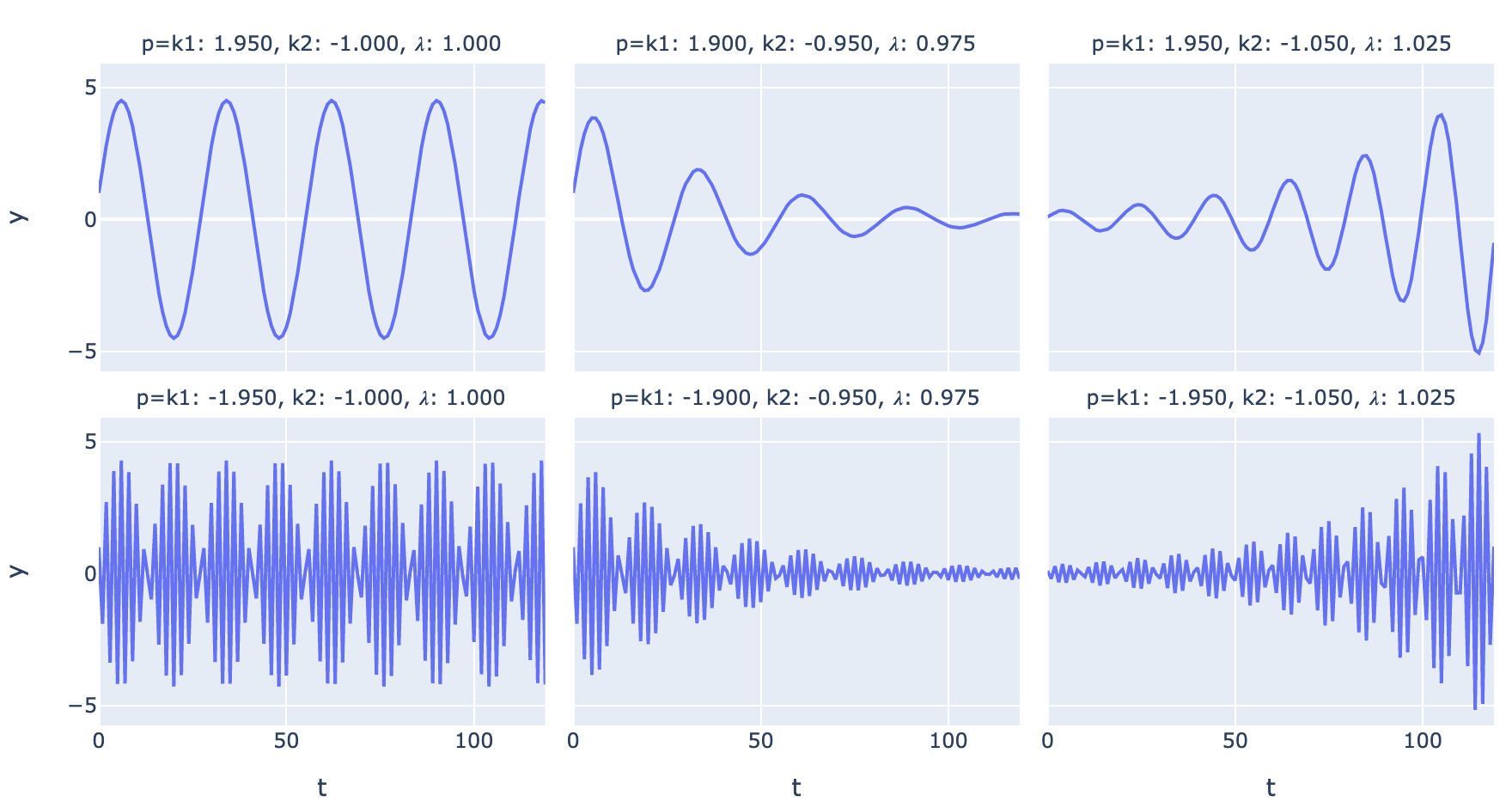
Comparing various regimes of periodic time series (\(\lambda\) here refers to the modulus of the complex roots):

Mapping the time series regime over values of \(k_1\) and \(k_2\), a parabola separates the region of real and complex roots:

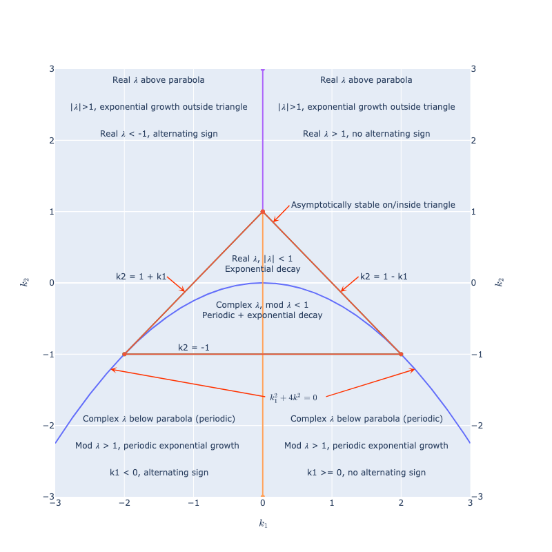
The parabola is the set of points where the quadratic discriminant is 0, below that we have a square root of a negative number, and complex \(\lambda\)s. Note that asymptotically the larger real \(\lambda\) in absolute value (or modulus) always dominates if its coefficient is nonzero.

If you disturb a stable physical system, 3 things can happen:

• It can return to the original stable state
• It can be unstable and blow up in some fashion
• It can oscillate.

A 2nd-order difference equation can model all 3 of these things, combining exponential growth or decay with periodicity.²

With higher order difference equations we can get more complicated shapes with an exponential trend or envelope and more complicated interacting periodic cycles.

5. Euler’s formula

So, if \(\lambda\) is complex, why is \(\lambda^t\) a trigonometric function, and how do 2 complex conjugate roots combine to yield a real cosine function?

To sort that out we will need Euler’s formula and representations of complex numbers in polar coordinates. If you are familiar with \(a + bi = r(\cos \theta + i \sin \theta) = r(e^{i \theta})\), then you can skip this section.

We can approximate any smooth function as a polynomial using Taylor series. Smooth means all the derivatives are continuous at all points in the interval over which we are performing the approximation.

If we know all the derivatives of some smooth non-polynomial function at some point, say 0, we can reverse-engineer the polynomial which would have the same value at that point and all the same derivatives. This is the Taylor series polynomial.

In fact, we can say that if two functions are smooth and have all the same derivatives at some point, then they are the same function. Smoothness and all derivatives being the same at some point are sufficient to say, at all points, because how can they ever deviate? (Not intended to be a valid mathematical proof, but it’s true, look it up.) So the infinite Taylor series expansion of any smooth function is the function itself.

If we construct the Taylor series for the exponential function, around 0, we get:

\[e^x = 1 + \frac{1}{1!} x + \frac{1}{2!} x^2 + \frac{1}{3!} x^3 + \frac{1}{4!} x^4 + \frac{1}{5!} x^5 \dots\]

All derivatives of \(e^x\) are \(e^x\), and \(e^0=1\) so all derivatives at 0 are 1.

If we construct the Taylor series for the \(\sin\) function,

• the derivative of \(\sin(x)\) is: \(\cos(x)\) (1 at x=0)
• the derivative of \(\cos(x)\) is: \(-\sin(x)\) (0 at x=0)
• the derivative of \(-\sin(x)\) is: \(-\cos(x)\) (-1 at x=0, natch)
• the derivative of \(-\cos(x)\) is: \(\sin(x)\) (0 at x=0; and repeat ad infinitum)

So the Taylor series for \(\sin(x)\) is

\[\sin x = 0 + \frac{1}{1!} x - 0 x^2 - \frac{1}{3!} x^3 + 0 x^4 + \frac{1}{5!} x^5\dots\]

and for \(\cos (x)\)

\[\cos x = 1 - 0 x - \frac{1}{2!} x^2 + 0 x^3 + \frac{1}{4!} x^4 - 0 x^5 \dots\]

Add these together and get:

\[\sin(x) + \cos(x) = 1 + \frac{1}{1!} x - \frac{1}{2!} x^2 - \frac{1}{3!} x^3 + \frac{1}{4!} x^4 + \frac{1}{5!} x^5 \dots\]

Plug in \(ix\) to our definition of \(e^x\):

\[e^{ix} = 1 + \frac{1}{1!} ix + \frac{1}{2!} i^2x^2 + \frac{1}{3!} i^3x^3 + \frac{1}{4!} i^4x^4 + \frac{1}{5!} i^5x^5 \dots\] \[= 1 + \frac{1}{1!} ix - \frac{1}{2!}x^2 - \frac{1}{3!} ix^3 + \frac{1}{4!}x^4 + \frac{1}{5!} ix^5 \dots\] \[= \cos(x) + i \sin(x)\]

This is Euler’s formula, \(e^{ix} = \cos(x) + i \sin(x)\).

Consider a representation of \(a +bi\) in the complex plane.

• Define \(r=\sqrt{a^2+b^2}\) (the modulus of a complex number)
• Define \(\theta = \tan^{-1}\frac{b}{a}\) (the argument, or the angle between the \(x\)-axis and \(a+bi\)).
• Then \(\cos \theta = \frac{a}{r}\) and \(\sin \theta = \frac{b}{r}\)
• Then \(a + bi = r(\cos \theta + i \sin \theta) = r(e^{i \theta})\), the polar coordinate representation of \(a + bi\).

6. Solving the 2nd-order difference equation with complex roots

This gets a bit gnarly. We have a 2nd-order difference equation:

\[y_t = k_1y_{t-1} + k_2y_{t-2}\]

We guess a solution is \(y_t = a\lambda^t\), and solve for \(\lambda\) using the characteristic equation:

\[-\lambda^2 + k_1 \lambda + k_2 = 0\]

We get 2 roots, and we solve using the initial conditions for

\[y_t = a_1 \lambda_1^t + a_2 \lambda_2^t\]

So, what if the \(\lambda\)s are complex? Then due to the form of the quadratic formula, we have:

\[\lambda_1 = \alpha+\beta i, \lambda_2 = \alpha-\beta i, \beta \ne 0\]

And

\[y_t = a_1 (\alpha+\beta i)^t + a_2 (\alpha-\beta i)^t\]

From the preceding section, we have the polar coordinate representation:

\[\alpha + \beta i = r e^{i\theta}\] \[\alpha - \beta i = r e^{-i\theta}\]

So we can substitute

\[y_t = a_1 (r e^{i\theta})^t + a_2 (r e^{-i\theta})^t\] \[y_t = a_1 r^t e^{i\theta t} + a_2 r^t e^{-i\theta t}\]

From the preceding section, we have \(e^{i \theta t} = \cos (\theta t) + i \sin (\theta t)\), so we can substitute:

\[y_t = a_1 r^t (\cos (\theta t) + i \sin (\theta t)) + a_2 r^t (\cos (\theta t) - i \sin (\theta t))\]

Redistributing so all the \(i\)s are together:

\[y_t = a_1 r^t \cos (\theta t) + i a_1 r^t \sin (\theta t)) + a_2 r^t \cos (\theta t) - i a_2 r^t \sin (\theta t)\] \[y_t = r^t [(a_1 + a_2) \cos (\theta t) + i (a_1 - a_2) \sin (\theta t)]\]

But \(y_t\) must be a real number. \(a_1\) and \(a_2\) may be complex. \(a_1 + a_2\) must be purely real. And \(a_1 - a_2\) must be purely imaginary, then we have a purely imaginary number times \(i\) and that imaginary part also cancels out. This is true if \(a_1\) and \(a_2\) are complex conjugates of the form \(a_1 = \alpha + \beta i\) and \(a_2 = \alpha - \beta i\).

If \(a_1\) and \(a_2\) are complex conjugates, then for some \(\rho\) and \(\omega\):

\[a_1 = \rho e^{i \omega} = \rho (\cos \omega + i \sin \omega)\] \[a_2 = \rho e^{-i \omega} = \rho (\cos \omega - i \sin \omega)\]

Substituting into the equation above:

\[y_t = r^t [(\rho (\cos \omega + i \sin \omega) + \rho (\cos \omega - i \sin \omega)) \cos (\theta t) + i (\rho (\cos \omega + i \sin \omega) - \rho (\cos \omega - i \sin \omega)) \sin (\theta t)]\] \[y_t = r^t [(\rho (2\cos \omega ) \cos (\theta t) + i (\rho (2 i \sin \omega)) \sin (\theta t)]\] \[= 2 \rho r^t [\cos \omega \cos (\theta t) - \sin \omega \sin (\theta t)]\]

by the identity \(\cos (a + b) = \cos \cos b - \sin a \sin b\) this is equal to

\[= 2 \rho r^t \cos (\theta t + \omega)\]

Hey, I said it was a bit gnarly. The part to remember is, when we have a complex conjugate root pair of the form \(\lambda = \alpha \pm \beta i\), we have a solution of the form:

\[y_t = \rho r^t \cos (\theta t + \omega)\]

where we can compute \(r\) and \(\theta\) from \(\alpha\) and \(\beta\) and then solve numerically for \(\rho\) and \(\omega\) using our initial conditions.

7. Writing an \(n\)th-order linear difference equation as a 1st-order matrix difference equation.

Consider our \(n\)th order linear difference equation:

\[y_t = k_1y_{t-1} + k_2y_{t-2} + k_3 y_{t-3} + \dots k_ny_{t-n}\]

Let’s specify the initial conditions as a state vector \(v_0\)

\[v_0 = \begin{bmatrix} y_{n-1} \\ y_{n-2} \\ . \\ . \\ y_{0} \end{bmatrix}\]

What matrix would we need to transform the state \(v_0\) to the state \(v_1\) with elements \([y_1, \dots, y_n]\)?

\[v_1 = \begin{bmatrix} k_1 & k_2 & k_3 & k_4 & \dots & k_{n-1} & k_n \\ 1 & 0 & 0 & 0 & \dots & 0 & 0 \\ 0 & 1 & 0 & 0 & \dots & 0 & 0 \\ 0 & 0 & 1 & 0 & \dots & 0 & 0 \\ . & . & . & . & & . & . \\ . & . & . & . & & . & . \\ 0 & 0 & 0 & . & \dots & 1 & 0 \\ \end{bmatrix} \cdot \begin{bmatrix} y_{n-1} \\ y_{n-2} \\ y_{n-3} \\ y_{n-4} \\ . \\ . \\ y_0 \end{bmatrix} = \begin{bmatrix} y_n \\ y_{n-1} \\ y_{n-2} \\ y_{n-3} \\ . \\ . \\ y_{1} \end{bmatrix}\]

The first row represents our difference equation, and applies the \(k_j\) coefficients to each element of \(v_0\), to create \(y_n\), the first element of \(v_1\).

The rest of the rows move each element of \(v\) down a row, and drop the last row. So each \(v_t\) has the \(n\) most recent elements of the time series available.

If we call our \(n \times n\) matrix \(F\), then we can say:

\[v_t = F v_{t-1}\]

and, raising \(F\) to the power \(t\) (repeatedly applying \(F\)):

\[v_t = F^t{v_0}\]

and:

\[v_t = F^jv_{t-j}\]

Suppose we compute eigenvectors of \(F\) as a matrix \(\xi\) and eigenvalues of \(F\) as a diagonal matrix \(D\). Then

\[F \cdot \xi = \xi \cdot D\]

This is the eigenvector equation in matrix form, it’s saying if you apply the transformation \(F\) to each of its eigenvectors \(\xi\), you get the product of the eigenvalues \(D\) and the eigenvectors \(\xi\). Suppose we set our initial conditions to an eigenvector of \(F\). Then at each timestep, \(y_t\) is the previous \(y_{t-1}\) multipled by the corresponding eigenvalue. So we can say

\[F^t \xi = D^t \xi\]

If \(y_0\) is an eigenvector of \(F\), then \(y_t\) evolves as a function of its eigenvalue raised to powers of \(t\). But guess what, we can express any initial condition as a linear combination of the eigenvectors. Then if we apply \(F\) to that linear combination, each eigenvector gets multiplied by its eigenvalue.

Multiply each side of the eigenvector equation by the inverse of the eigenvectors (assuming invertible):

\[F \cdot \xi \xi^{-1} = F = \xi D \xi^{-1}\]

This is the eigendecomposition. It says that there is a basis \(\xi\) (the eigenvectors) under which the transformation \(F\) is described by a diagonal matrix of its eigenvalues.

Using this basis we can say

\[v_t = F^tv_0 = (\xi D \xi^{-1})^t {v_0} = \xi D^t \xi^{-1} {v_0}\]

because:

\[(\xi D \xi^{-1})^t = \xi D \xi^{-1} \xi D \xi^{-1} \xi D \xi^{-1} \cdots\]

and the middle \(\xi^{-1}\xi\)s all cancel out leaving \(\xi D^t \xi^{-1}\)

We can interpret the matrix representation \(v_t = F^t v_0 = \xi D^t \xi^{-1} v_0\) in the following way:

• \(\xi^{-1} v_0\) represents the initial conditions with a change of coordinates into the eigenvector basis \(\xi\).

• Multiplying by \(D^t\) applies the simple dynamics in this new basis.

• Finally multiplying by \(\xi\) changes our coordinate system back to the standard basis.

• When we change to the basis of the eigenvectors \(\xi\), our difference equation has simple dynamics governed by the eigenvalues and powers of \(t\).

Which is saying that the evolution of \(v_t\) over time is the result of applying a power to the eigenvalues in the basis \(\xi^{-1}\).

Recall that the eigenvalues are the roots of the characteristic polynomial of the matrix, like our \(\lambda\)s are the roots of the \(n\)th-degree characteristic polynomial of the \(n\)th-order difference equation.

Lo and behold, if we calculate the characteristic polynomial of our matrix as \(\det(F - \lambda I_n)\), we will find the characteristic polynomial of our difference equation.

This leads to a 2nd method of solving any \(n\)th-order difference equation:

1. Write the \(n\)th-order linear difference equation as a 1st-order matrix difference equation \(F\), so that \(v_t = F v_{t-1}\)

2. Solve for the eigenvalues of \(F\), the roots of the characteristic polynomial \(\det(F - \lambda I_n)\).

3. Solve the system of \(n\) linear equations given by:

\[\begin{bmatrix} 1 & 1 & 1 & \dots & 1 \\ \lambda_1 & \lambda_2 & \lambda_3 & \dots & \lambda_n \\ \lambda_1^2 & \lambda_2^2 & \lambda_3^2& \dots & \lambda_n^2 \\ . \\ . \\ . \\ \lambda_1^{n-1} & \lambda_2^{n-1} & \lambda_3^{n-1}& \dots & \lambda_n^{n-1} \\ \end{bmatrix} \begin{bmatrix} a_1 \\ a_2 \\ a_3 \\ . \\ . \\ . \\ a_{n} \\ \end{bmatrix} = \begin{bmatrix} y_0 \\ y_1 \\ y_2 \\ . \\ . \\ . \\ y_{n-1} \end{bmatrix}\]

or

\[V \cdot \bf{a} = \bf{v_0}\]

(Note that \(\bf{v_0}\) is in reverse order from the way we apply the \(F\). Also, \(V\) is known as the Vandermonde matrix.)

When we solve this system of equations, we solve for \(a\)s that capture the eigenvectors \(\xi\) and \(\xi^{-1}\) and the boundary counditions.

8. Summing up:

Given an \(n\)th-order difference equation of the form:

\[y_t = k_1y_{t-1} + k_2y_{t-2} + k_3 y_{t-3} + \dots k_ny_{t-n}\]

• Find the roots of the characteristic equation

\[- \lambda^n + k_1 \lambda^{n-1} + k_2 \lambda^{n-2} + \dots + k_{n-1} \lambda + k_n= 0\]

• Or, find the matrix representation \(F\), and factor \(F\) using the eigendecomposition a/k/a diagonalization a/k/a spectral decomposition:

\[F = \xi D \xi^{-1}\]

• Here, \(D\) is a diagonal matrix of \(\lambda\)s, with a combination of possible real roots and pairs of complex roots.

• Each real \(\lambda\) corresponds to an exponential growth / decay solution with no periodicity, \(y_t = \lambda^t\).

• Each pair of complex roots corresponds to a periodic component within an exponential growth / decay envelope, \(y_t = \rho r^t \cos (\theta t + \omega)\). (you can see why eigendecomposition is also referred to as spectral decomposition.)

• A closed-form expression is \(y_t = D^t \bf{a}\), a linear combination of the \(\lambda^t\)s. We use our initial conditions to solve for the numeric value of \(\bf{a}\). Each pair of complex roots is composed of complex conjugates, as are the corresponding \(a\)s, so all the \(i\)s cancel out to give a real cosine expression.

• Asymptotically, the root (eigenvalue) with largest absolute value (modulus) will dominate. If it is larger than 1 in absolute value (modulus) our time series diverges. If it is less than 1 in absolute value (modulus) our time series goes to 0. If it is equal to 1 in absolute value (modulus) our time series is neutrally stable in the region of the initial conditions.

There’s probably a simple way to solve the cosine expression given initial conditions. When I learn it/figure it out I’ll update.

Some tutorials on time series dive straight into ARIMA without asking what a time series is and what types of processes ARIMA can model.

Now we know. \(n\)th-degree difference equations can model any process that generates a time series with an exponential trend or envelope (the real eigenvalues), and multiple cyclical seasonal components (the conjugate pairs of complex eigenvalues). When we add a little more complexity, ARIMA processes can model combinations of trends and cycles and stochastic disturbances that resolve over multiple time periods, but not arbitrary functions or even arbitrary polynomials.

If we have a time series, we can do exploratory data analysis to see if it might come from this type of process, parameterize it to fit our data, and generate forecasts. Hopefully the next post will do a standard ARIMA model, and then we will move on to a deep learning model.

If you made it this far, congratulations!

Code is in GitHub.

Run in Google Colab

References

• This mostly follows Hamilton, James D. Time Series Analysis, chapter 1. It’s pretty dense and assumes solid linear algebra. Basically I tried working it out and explaining it to myself and this post is the result.
• Steve Brunton a/k/a Eigensteve has some excellent videos on dynamic systems in general (not time series specifically but a first-order linear difference equation becomes a first-order linear ordinary differential equation as the size of the timesteps goes to 0. Higher order difference equations involve higher order lags, while higher-order ODEs involve higher-order derivatives, I’m not 100% clear on how they correspond although they can describe similar processes).