Are long term asset class relationships stable?
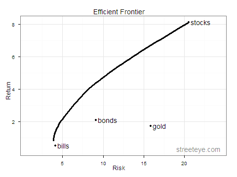
Last week, we looked at gold as part of a long-term asset allocation. I was curious about how stable those relationships would be over time, so I ran the same plots, starting from different inflection points.
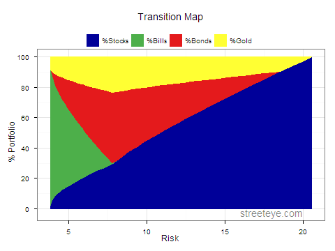
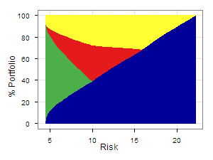
(The transition map shows you the composition of the maximum return portfolio for each level of risk.)
1946-2010, Post-war, since Bretton Woods:
1972-2010, Post-war, post-gold standard:
1982-2010, Era of disinflation, globalization:
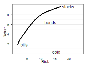
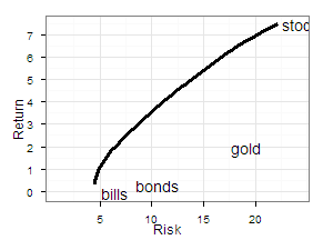
This is interesting, since it shows how poorly gold has performed since 1982, an era of low inflation, the dollar standard, and decreasing holdings of gold by central banks and investors.
Note that this does not include the 37% decline in real gold prices from 1980-1981, as the gold bull market ended amid still-high inflation.
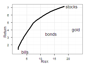
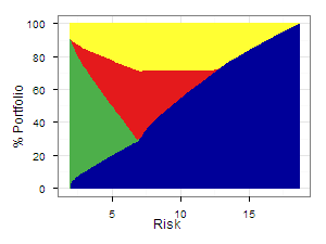
Let’s compare the pre-1982 era. Note the shift down and to the right: a less favorable tradeoff of lower returns and higher risks.
1928-1981:
Take-aways:
- The shape of the efficient frontier has been mostly fairly stable over the long term, with gold offering high risk, low real return, little correlation with other assets, and adding value to most portfolios.
- From 1982 until recently, the environment was unusually favorable for financial assets in general, extremely favorable for bonds, and unusually poor for gold.
R code for the masochists:
1 2 3 4 5 6 7 8 9 10 11 12 13 14 15 16 17 18 19 20 21 22 23 24 25 26 27 28 29 30 31 32 33 34 35 36 37 38 39 40 41 42 43 44 45 46 47 48 49 50 51 52 53 54 55 56 57 58 59 60 61 62 63 64 65 66 67 68 69 70 71 72 73 74 75 76 77 78 79 80 81 82 83 84 85 86 87 88 89 90 91 92 93 94 95 96 97 98 99 100 101 102 103 104 105 106 107 108 109 110 111 112 113 114 115 116 117 118 119 120 121 122 123 124 125 126 127 128 129 130 131 132 133 134 135 136 137 138 139 140 141 142 143 144 145 146 147 148 149 150 151 152 153 154 155 156 157 158 159 160 161 162 163 164 165 166 167 168 169 170 171 172 173 174 175 176 177 178 179 180 181 182 183 184 185 186 187 188 189 190 191 192 193 194 195 196 197 198 199 200 201 202 203 204 205 206 207 208 209 210 211 212 213 214 215 216 217 218 219 220 221 222 223 224 225 226 227 228 229 230 231 232 233 234 235 236 237 238 239 240 241 242 243 244 245 246 247 248 249 250 251 252 253 254 255 256 257 258 259 260 261 262 263 264 265 266 267 268 269 270 271 272 273 274 275 276 277 278 279 280 281 282 283 284 285 286 287 288 289 290 291 292 293 294 295 296 297 298 299 300 301 302 303 304 305 306 307 308 309 310 311 312 313 314 315 316 317 318 319 320 321 322 323 324 325 326 327 328 329 330 331 332 333 334 335 336 337 338 339 340 341 342 343 344 345 346 347 348 349 350 351 352 353 354 355 356 357 358 359 360 361 362 363 |
# install.packages('quantmod') require(quantmod) # install.packages('lpSolve') require(lpSolve) # install.packages('quadprog') require(quadprog) # install.packages('ggplot2') require(ggplot2) require(reshape) # define functions ################################################################# # use linear programming to find maximum return portfolio (100% highest return asset) ################################################################# runlp <- function ( returns ) { # find maximum return portfolio (rightmost point of efficient frontier) # will be 100% of highest return asset # maximize # w1 * stocks return +w2 *bills +w3*bonds + w4 * gold # subject to 0 <= w <= 1 for each w # will pick highest return asset with w=1 # skipping >0 constraint, no negative return assets, so not binding opt.objective <- apply(returns, 2, mean) # should use length(objective) to populate matrix nAssets <- length(returns) ones = rep (1, nAssets) zeros = rep (, nAssets) # constrain sum of weights to 1 constraintlist = ones operatorlist = c("=") rhslist = c(1) # constrain each weight >= 0 for(i in 1:nAssets) { newconstraint = zeros newconstraint[i]=1 constraintlist = c(constraintlist, newconstraint) operatorlist = c(operatorlist, ">=") rhslist = c(rhslist, ) } # Example # opt.constraints <- matrix (c(1, 1, 1, 1, # constrain sum of weights to 1 # 1, 0, 0, 0, # constrain w1 <= 1 # 0, 1, 0, 0, # constrain w2 <= 1 # 0, 0, 1, 0, # constrain w3 <= 1 # 0, 0, 0, 1) # constrain w4 <= 1 # , nrow=5, byrow=TRUE) opt.constraints <- matrix (constraintlist, nrow=nAssets+1, byrow=TRUE) opt.operator <- operatorlist opt.rhs <- rhslist opt.dir="max" tmpsolution = lp (direction = opt.dir, opt.objective, opt.constraints, opt.operator, opt.rhs) sol= c() # portfolio weights for max return portfolio sol$wts=tmpsolution$solution # return for max return portfolio sol$ret=tmpsolution$objval # compute return covariance matrix to determine volatility of this portfolio sol$covmatrix = cov(returns, use = 'complete.obs', method = 'pearson') # multiply weights x covariances x weights, gives variance sol$var = sol$wts %*% sol$covmatrix %*% sol$wts # square root gives standard deviation (volatility) sol$vol = sqrt(sol$var) return (sol) } runqp <- function ( returns, hurdle= ) { ################################################################# # find minimum volatility portfolio ################################################################# # minimize variance: w %*% covmatrix %*% t(w) # subject to sum of ws = 1 # subject to each w >= 0 # subject to each return >= hurdle # solution.minvol <- solve.QP(covmatrix, zeros, t(opt.constraints), opt.rhs, meq = opt.meq) # first 2 parameters covmatrix, zeros define function to be minimized # if zeros is all 0s, the function minimized ends up equal to port variance / 2 # opt.constraints is the left hand side of the constraints, ie the cs in # c1 w1 + c2 w2 ... + cn wn = K # opt.rhs is the Ks in the above equation # meq means the first meq rows are 'equals' constraints, remainder are >= constraints # if you want to do a <= constraint, multiply by -1 to make it a >= constraint # does not appear to accept 0 RHS, so we make it a tiny number> 0 # compute expected returns meanreturns <- apply(returns, 2, mean) # compute covariance matrix covmatrix = cov(returns, use = 'complete.obs', method = 'pearson') nAssets <- length(returns) nObs <- length(returns$stocks) ones = rep (1, nAssets) zeros = rep (, nAssets) # constrain sum of weights to 1 constraintlist = ones rhslist = c(1) # constrain each weight >= 0 for(i in 1:nAssets) { newconstraint = zeros newconstraint[i]=1 constraintlist = c(constraintlist, newconstraint) rhslist = c(rhslist, ) } # constrain return >= hurdle constraintlist = c(constraintlist, meanreturns) rhslist = c(rhslist, hurdle) # example # opt.constraints <- matrix (c(1, 1, 1, 1, # sum of weights =1 # 1, 0, 0, 0, # w1 >= 0 # 0, 1, 0, 0, # w2 >= 0 # 0, 0, 1, 0, # w3 >= 0 # 0, 0, 0, 1) # w4 >= 0 # , nrow=5, byrow=TRUE) # opt.rhs <- matrix(c(1, 0.000001, 0.000001, 0.000001, 0.000001)) # opt.constraints = rbind(opt.constraints, meanreturns) # opt.rhs=rbind(opt.rhs, hurdle) opt.constraints <- matrix (constraintlist, nrow=nAssets+2, byrow=TRUE) opt.rhs <- opt.rhs <- matrix(rhslist) opt.meq <- 1 # first constraint is '=', rest are '>=' zeros <- array(, dim = c(nAssets,1)) tmpsolution <- solve.QP(covmatrix, zeros, t(opt.constraints), opt.rhs, meq = opt.meq) sol= c() sol$wts = tmpsolution$solution sol$var = tmpsolution$value *2 sol$ret = meanreturns %*% sol$wts sol$vol = sqrt(sol$var) return(sol) } loopqp <- function (minvol, maxret, numtrials) { ################################################################# # loop and run a minimum volatility optimization for each return level from 2-49 ################################################################# # put minreturn portfolio in return series for min return, index =1 out.ret=c(minvol$ret) out.vol=c(minvol$vol) out.stocks=c(minvol$wts[1]) out.bills=c(minvol$wts[2]) out.bonds=c(minvol$wts[3]) out.gold=c(minvol$wts[4]) lowreturn <- minvol$ret highreturn <- maxret$ret minreturns <- seq(lowreturn, highreturn, length.out=numtrials) for(i in 2:(length(minreturns) - 1)) { tmpsol <- runqp(freal,minreturns[i]) tmp.wts = tmpsol$wts tmp.var = tmpsol$var out.ret[i] = realreturns %*% tmp.wts out.vol[i] = sqrt(tmp.var) out.stocks[i]=tmp.wts[1] out.bills[i]=tmp.wts[2] out.bonds[i]=tmp.wts[3] out.gold[i]=tmp.wts[4] } # put maxreturn portfolio in return series for max return out.ret[numtrials]=c(maxret$ret) out.vol[numtrials]=c(maxret$vol) out.stocks[numtrials]=c(maxret$wts[1]) out.bills[numtrials]=c(maxret$wts[2]) out.bonds[numtrials]=c(maxret$wts[3]) out.gold[numtrials]=c(maxret$wts[4]) efrontier=data.frame(out.ret*100) efrontier$vol=out.vol*100 efrontier$stocks=out.stocks*100 efrontier$bills=out.bills*100 efrontier$bonds=out.bonds*100 efrontier$gold=out.gold*100 names(efrontier) = c("Return", "Risk", "%Stocks", "%Bills", "%Bonds", "%Gold") return(efrontier) } ############################################################ # charts ############################################################ plot_efrontier <- function (efrontier, returns, sds, apoints) { ggplot(data=efrontier, aes(x=Risk, y=Return)) + # opts(title="Efficient Frontier") + theme_bw() + geom_line(size=1.4) + geom_point(aes(x=apoints$sds, y=apoints$returns)) + scale_x_continuous(limits=c(1,24)) + # could loop through efrontier names annotate("text", apoints[1,1], apoints[1,2],label=" stocks", hjust=) + annotate("text", apoints[2,1], apoints[2,2],label=" bills", hjust=) + annotate("text", apoints[3,1], apoints[3,2],label=" bonds", hjust=) + annotate("text", apoints[4,1], apoints[4,2],label=" gold", hjust=) # annotate("text", 19,0.3,label="streeteye.com", hjust=0, alpha=0.5) } plot_transitionmap <- function (efrontier, returns, sds) { # define colors dvblue = "#000099" dvred = "#e41a1c" dvgreen = "#4daf4a" dvpurple = "#984ea3" dvorange = "#ff7f00" dvyellow = "#ffff33" dvgray="#666666" efrontier.m = melt(efrontier, id ='Risk') ggplot(data=efrontier.m, aes(x=Risk, y=value, colour=variable, fill=variable)) + theme_bw() + theme(legend.position="top", legend.direction="horizontal") + ylab('% Portfolio') + geom_area() + scale_colour_manual("", breaks=c("%Stocks", "%Bills", "%Bonds","%Gold"), values = c(dvblue,dvgreen,dvred,dvyellow), labels=c('%Stocks', '%Bills','%Bonds','%Gold')) + scale_fill_manual("", breaks=c("%Stocks", "%Bills", "%Bonds","%Gold"), values = c(dvblue,dvgreen,dvred,dvyellow), labels=c('%Stocks', '%Bills','%Bonds','%Gold')) # annotate("text", 16,-2.5,label="streeteye.com", hjust=0, alpha=0.5) } ################################################################# # Create some data ################################################################# # not used in abbreviated example, but useful for reporting startYear = 1928 endYear = 2010 YEARS =startYear:endYear # nominal returns # nominal returns SP500 = c(0.4381,-0.083,-0.2512,-0.4384,-0.0864,0.4998,-0.0119,0.4674,0.3194,-0.3534,0.2928,-0.011, -0.1067,-0.1277,0.1917,0.2506,0.1903,0.3582,-0.0843,0.052,0.057,0.183,0.3081,0.2368,0.1815, -0.0121,0.5256,0.326,0.0744,-0.1046,0.4372,0.1206,0.0034,0.2664,-0.0881,0.2261,0.1642,0.124, -0.0997,0.238,0.1081,-0.0824,0.0356,0.1422,0.1876,-0.1431,-0.259,0.37,0.2383,-0.0698,0.0651, 0.1852,0.3174,-0.047,0.2042,0.2234,0.0615,0.3124,0.1849,0.0581,0.1654,0.3148,-0.0306,0.3023, 0.0749,0.0997,0.0133,0.372,0.2268,0.331,0.2834,0.2089,-0.0903,-0.1185,-0.2197,0.2836,0.1074, 0.0483,0.1561,0.0548,-0.3655,0.2594,0.1482,0.021,0.1589,0.3215,0.1348) BILLS = c(0.0308,0.0316,0.0455,0.0231,0.0107,0.0096,0.0032,0.0018,0.0017,0.003,0.0008,0.0004, 0.0003,0.0008,0.0034,0.0038,0.0038,0.0038,0.0038,0.0057,0.0102,0.011,0.0117,0.0148, 0.0167,0.0189,0.0096,0.0166,0.0256,0.0323,0.0178,0.0326,0.0305,0.0227,0.0278,0.0311, 0.0351,0.039,0.0484,0.0433,0.0526,0.0656,0.0669,0.0454,0.0395,0.0673,0.0778,0.0599, 0.0497,0.0513,0.0693,0.0994,0.1122,0.143,0.1101,0.0845,0.0961,0.0749,0.0604,0.0572, 0.0645,0.0811,0.0755,0.0561,0.0341,0.0298,0.0399,0.0552,0.0502,0.0505,0.0473,0.0451, 0.0576,0.0367,0.0166,0.0103,0.0123,0.0301,0.0468,0.0464,0.0159,0.0014,0.0013,0.0003, 0.0005,0.0007,0.0005) BONDS=c(0.0084,0.042,0.0454,-0.0256,0.0879,0.0186,0.0796,0.0447,0.0502,0.0138,0.0421,0.0441, 0.054,-0.0202,0.0229,0.0249,0.0258,0.038,0.0313,0.0092,0.0195,0.0466,0.0043,-0.003, 0.0227,0.0414,0.0329,-0.0134,-0.0226,0.068,-0.021,-0.0265,0.1164,0.0206,0.0569,0.0168, 0.0373,0.0072,0.0291,-0.0158,0.0327,-0.0501,0.1675,0.0979,0.0282,0.0366,0.0199,0.0361, 0.1598,0.0129,-0.0078,0.0067,-0.0299,0.082,0.3281,0.032,0.1373,0.2571,0.2428,-0.0496, 0.0822,0.1769,0.0624,0.15,0.0936,0.1421,-0.0804,0.2348,0.0143,0.0994,0.1492,-0.0825, 0.1666,0.0557,0.1512,0.0038,0.0449,0.0287,0.0196,0.1021,0.201,-0.1112,0.0846,0.1604, 0.0297,-0.091,0.1075) CPI=c(-0.0115607,0.005848,-0.0639535,-0.0931677,-0.1027397,0.0076336,0.0151515,0.0298507, 0.0144928,0.0285714,-0.0277778,,0.0071429,0.0992908,0.0903226,0.0295858,0.0229885, 0.0224719,0.1813187,0.0883721,0.0299145,-0.0207469,0.059322,0.06,0.0075472,0.0074906, -0.0074349,0.0037453,0.0298507,0.0289855,0.0176056,0.017301,0.0136054,0.0067114,0.0133333, 0.0164474,0.0097087,0.0192308,0.0345912,0.0303951,0.0471976,0.0619718,0.0557029,0.0326633, 0.0340633,0.0870588,0.1233766,0.0693642,0.0486486,0.0670103,0.0901771,0.1329394,0.125163, 0.0892236,0.0382979,0.0379098,0.0394867,0.0379867,0.010979,0.0443439,0.0441941,0.046473, 0.0610626,0.0306428,0.0290065,0.0274841,0.026749,0.0253841,0.0332248,0.017024,0.016119, 0.0268456,0.0338681,0.0155172,0.0237691,0.0187949,0.0325556,0.0341566,0.0254065,0.0408127, 0.0009141,0.0272133,0.0149572,0.03,0.017,0.015,0.008) GOLD = c(,,,,,0.563618771,0.082920792, ,,,,,-0.014285714,0.028985507,, 0.028169014,-0.006849315,0.027586207,0.026845638,0.124183007,-0.023255814,-0.035714286, -0.00617284,-0.00621118,-0.0325,-0.082687339,-0.007042254,-0.002836879,0.001422475, 0.001420455,,,0.035460993,-0.02739726,-0.004225352,-0.002828854, 0.002836879,0.004243281,-0.002816901,0.002824859,0.225352113,-0.057471264,-0.051219512, 0.146529563,0.431390135,0.667919799,0.725864012,-0.242041683,-0.03962955,0.204305898, 0.291744258,1.205670351,0.296078431,-0.327618087,0.1175,-0.149888143,-0.189473684, 0.061688312,0.195412844,0.244563827,-0.156937307,-0.022308911,-0.036907731,-0.085577421, -0.057057907,0.176426426,-0.021697511,0.009784736,-0.046511628,-0.222086721,0.005748128, 0.005368895,-0.060637382,0.014120668,0.23960217,0.217359592,0.04397843,0.17768595, 0.231968811,0.319224684,0.043178411,0.250359299,0.292413793,0.089292067,0.082625735, -0.273303167,0.00124533 ) # truncate here, e.g. # 1928 - 2014 - 87 years # 1946 - 2010 - 65 years # lop off first 18 years # SP500=SP500[19:87] # BILLS=BILLS[19:87] # BONDS=BONDS[19:87] # GOLD=GOLD[19:87] # CPI=CPI[19:87] # 1972 - 2014 - 43 years # 1982 - 2014 - 33 years # put into a data frame (matrix) fnominal=data.frame(stocks=SP500, bills=BILLS, bonds=BONDS, gold=GOLD, CPI=CPI) freal=data.frame(stocks=SP500-CPI, bills=BILLS-CPI, bonds=BONDS-CPI, gold=GOLD-CPI) # compute real returns realreturns = apply(freal, 2, mean) realreturnspct = realreturns*100 # print them realreturnspct # compute real volatility (standard deviation of real returns) realsds = apply(freal, 2, sd) realsdspct = realsds*100 # print them realsdspct maxret <- runlp(freal) minvol <- runqp(freal,) # generate a sequence of 50 evenly spaced returns between min var return and max return efrontier = loopqp(minvol, maxret, 50) apoints <- data.frame(realsdspct) apoints$returns <- realreturnspct names(apoints) = c("Risk", "Return") png(filename="/temp/ltg11.png", width=300, height=225, units="px") plot_efrontier(efrontier, realreturnspct, realsdspct, apoints) dev.off() keep=c("Risk", "%Stocks","%Bills","%Bonds","%Gold") png(filename="/temp/ltg12.png", width=300, height=225, units="px") plot_transitionmap(efrontier[keep], realreturnspct, realsdspct) dev.off() |
