Portfolio Optimization and Efficient Frontiers in R
If you want to frustrate someone for a day, give them a program. If you want to frustrate them for a lifetime, teach them how to program.
A brief overview of how to use R to generate the analysis and plots in the most recent post, Gold as Part of a Long-Run Asset Allocation, using R, and code shared at Systematic Investor.
R is a powerful open-source statistical analysis package, a free version of products like SPSS, SAS, S-plus, to some extent MatLab (MatLab may target mathematical modeling more generally, not just statistics). R doesn’t do symbolic math, ie algebraic formulas, integration, differentiation etc., for that you can use Mathematica, Maple, Sage, Maxima.
R is basically Excel on steroids. R is very powerful, and beating your head against the wall using R will open many doors to… more powerful ways to beat your head against the wall using R.
Step 1. Install R. Get it here. Also recommended _ install RStudio. This gives you an integrated development environment, lets you browse history, data objects, help, etc.
Step 2. Let’s get some data and plot a quick chart.
_ Launch RStudio (or R)
_ install ‘quantmod’ package (Quantitative Financial Modelling & Trading Framework for R). This provides the ability to download financial data, do backtesting, other modeling functionality. One of R’s biggest strengths is that whatever you want to do, someone has probably already developed a module to do it, and it’s already in the CRAN archive, one command away from being installed. (The downside is that often there is more than one way to do it, and it’s hard to figure out the best way, for instance multiple timeseries and graphics modules)
1 2 3 4 5 6 7 8 9 10 11 12 13 14 |
> install.packages("quantmod") > # load library > require(quantmod) > # some ETFs we might choose for a portfolio: > symbols = c('SPY','IWM','EFA','EEM','AGG','IYR','GLD') > # these are, respectiviely > symbol.names = c('S&P 500','Russell 2000','Europe, Australasia, Far East developed', 'Emerging Markets','Agg bond','REIT','Gold') > # download data using quantmod > getSymbols(symbols, from = '2003-01-01', auto.assign = TRUE) > # run a chart > candleChart(SPY,theme='white', type='candles') > # run a chart with shorter history so we can see better > SPY_6MO<-SPY['2011-06-01::'] > candleChart(SPY_6MO,theme='white', type='candles') |
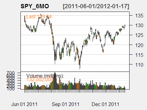
You should see something like the below. More on quantmod charts here.
For documentation on quantmod and other functions, you can get help with
1 2 3 |
> ?getSymbols > ?candleChart > ?quantmod |
…etc. (remember, R is case-sensitive).
3. Data setup
Parts 3 and onward use the code in this longtermgold.r file.
Here, we create a data frame (matrix) of real returns, and report basic data on it.
1 2 3 4 5 6 7 8 9 10 11 12 13 14 15 16 17 18 19 20 21 22 23 24 25 26 27 28 29 30 31 32 33 34 35 36 37 38 39 40 41 42 43 44 45 46 47 48 49 50 51 52 53 54 55 56 57 58 59 60 61 |
> # nominal returns > SP500 = c(0.4381,-0.083,-0.2512,-0.4384,-0.0864,0.4998,-0.0119,0.4674,0.3194,-0.3534,0.2928, -0.011,-0.1067,-0.1277,0.1917,0.2506,0.1903,0.3582,-0.0843,0.052,0.057,0.183,0.3081,0.2368, 0.1815,-0.0121,0.5256,0.326,0.0744,-0.1046,0.4372,0.1206,0.0034,0.2664,-0.0881,0.2261,0.1642, 0.124,-0.0997,0.238,0.1081,-0.0824,0.0356,0.1422,0.1876,-0.1431,-0.259,0.370,0.2383,-0.0698, 0.0651,0.1852,0.3174,-0.047,0.2042,0.2234,0.0615,0.3124,0.1849,0.0581,0.1654,0.3148,-0.0306, 0.3023,0.0749,0.0997,0.0133,0.372,0.2382,0.3186,0.2834,0.2089,-0.0903,-0.1185,-0.2197,0.2836, 0.1074,0.0483,0.1561,0.0548,-0.3658,0.2592,0.148600) > BILLS = c(0.0308,0.0316,0.0455,0.0231,0.0107,0.0096,0.0032,0.0018,0.0017,0.003,0.0008,0.0004, 0.0003,0.0008,0.0034,0.0038,0.0038,0.0038,0.0038,0.0057,0.0102,0.011,0.0117,0.0148,0.0167, 0.0189,0.0096,0.0166,0.0256,0.0323,0.0178,0.0326,0.0305,0.0227,0.0278,0.0311,0.0351,0.039, 0.0484,0.0433,0.0526,0.0656,0.0669,0.0454,0.0395,0.0673,0.0778,0.0599,0.0497,0.0513,0.0693, 0.0994,0.1122,0.143,0.1101,0.0845,0.0961,0.0749,0.0604,0.0572,0.0645,0.0811,0.0755,0.0561, 0.0341,0.0298,0.0399,0.0552,0.0502,0.0505,0.0473,0.0451,0.0576,0.0367,0.0166,0.0103,0.0123, 0.0301,0.0468,0.0464,0.0159,0.0014,0.001300) > BONDS=c(0.0084,0.042,0.0454,-0.0256,0.0879,0.0186,0.0796,0.0447,0.0502,0.0138,0.0421,0.0441, 0.054,-0.0202,0.0229,0.0249,0.0258,0.038,0.0313,0.0092,0.0195,0.0466,0.0043,-0.003,0.0227, 0.0414,0.0329,-0.0134,-0.0226,0.068,-0.021,-0.0265,0.1164,0.0206,0.0569,0.0168,0.0373,0.0072, 0.0291,-0.0158,0.0327,-0.0501,0.1675,0.0979,0.0282,0.0366,0.0199,0.0361,0.1598,0.0129,-0.0078, 0.0067,-0.0299,0.082,0.3281,0.032,0.1373,0.2571,0.2428,-0.0496,0.0822,0.1769,0.0624,0.150, 0.0936,0.1421,-0.0804,0.2348,0.0143,0.0994,0.1492,-0.0825,0.1666,0.0557,0.1512,0.0038,0.0449, 0.0287,0.0196,0.1021,0.201,-0.1112,0.084600) > CPI=c(-0.0115607,0.005848,-0.0639535,-0.0931677,-0.1027397,0.0076336,0.0151515,0.0298507, 0.0144928,0.0285714,-0.0277778,0.0000,0.0071429,0.0992908,0.0903226,0.0295858,0.0229885, 0.0224719,0.1813187,0.0883721,0.0299145,-0.0207469,0.059322,0.0600,0.0075472,0.0074906, -0.0074349,0.0037453,0.0298507,0.0289855,0.0176056,0.017301,0.0136054,0.0067114,0.0133333, 0.0164474,0.0097087,0.0192308,0.0345912,0.0303951,0.0471976,0.0619718,0.0557029,0.0326633, 0.0340633,0.0870588,0.1233766,0.0693642,0.0486486,0.0670103,0.0901771,0.1329394,0.125163, 0.0892236,0.0382979,0.0379098,0.0394867,0.0379867,0.010979,0.0443439,0.0441941,0.046473, 0.0610626,0.0306428,0.0290065,0.0274841,0.026749,0.0253841,0.0332248,0.017024,0.016119, 0.0268456,0.0338681,0.0155172,0.0237691,0.0187949,0.0325556,0.0341566,0.0254065,0.0408127, 0.0009141,0.0272133,0.0149572) > GOLD = c(0.000000000,0.000000000,0.000000000,0.000000000,0.000000000,0.447002860,0.079661828, 0.000000000,0.000000000,0.000000000,0.000000000,0.000000000,-0.014388737,0.028573372,0.000000000, 0.027779564,-0.006872879,0.027212564,0.026491615,0.117056555,-0.023530497,-0.036367644, -0.006191970,-0.006230550,-0.033039854,-0.086306904,-0.007067167,-0.002840911,0.001421464, 0.001419447,0.000000000,0.000000000,0.034846731,-0.027779564,-0.004234304,-0.002832863, 0.002832863,0.004234304,-0.002820876,0.002820876,0.203228242,-0.059188871,-0.052577816, 0.136739608,0.358646094,0.511577221,0.545727802,-0.132280611,-0.253090628,0.168898536, 0.265477915,0.464157559,0.689884535,-0.285505793,-0.201637346,0.120144312,-0.163629424, -0.127202258,0.149181164,0.192236014,-0.020385757,-0.134512586,0.005221944,-0.058998341, -0.051002554,0.045462374,0.064538521,0.002600782,0.010336009,-0.155436854,-0.121167134, -0.052185753,0.000000000,-0.028987537,0.133990846,0.157360955,0.119003292,0.084161792, 0.308209839,0.142551544,0.220855221,0.110501915,0.228258652) > # put into a data frame (matrix) > fnominal=data.frame(stocks=SP500, bills=BILLS, bonds=BONDS, gold=GOLD, CPI=CPI) > freal=data.frame(stocks=SP500-CPI, bills=BILLS-CPI, bonds=BONDS-CPI, gold=GOLD-CPI) > # compute real returns > realreturns = apply(freal, 2, mean) > realreturnspct = realreturns*100 > # print them > realreturnspct stocks bills bonds gold 8.1255600 0.5107407 2.0921865 1.7287079 > # compute real volatility (standard deviation of real returns) > realsds = apply(freal, 2, sd) > realsdspct = realsds*100 > # print them > realsdspct stocks bills bonds gold 20.556871 4.116415 9.095301 15.834720 |
4. The Easy Way
There’s an easy way and a hard way. For the easy way, we will use the code generously shared by Systematic Investor. For the hard way, we’ll go through the same steps, but writing our own code (inspired by the Systematic Investor Toolbox).
1 2 3 4 5 6 7 8 9 10 11 12 13 14 15 16 17 18 19 20 21 22 23 24 25 26 27 28 29 30 31 32 33 34 35 36 37 38 39 40 41 |
> # put input assumption in suitable format for Systematic Investor Toolbox > ia = list() > ia$n = length(freal) > ia$annual.factor = 1 > ia$symbols = names(freal) > ia$symbol.names = names(freal) > ia$hist.returns = freal > > ia$arithmetic.return = apply(ia$hist.returns, 2, mean, na.rm = T) > ia$arithmetic.return = (1 + ia$arithmetic.return)^ia$annual.factor - 1 > ia$geometric.return = apply(ia$hist.returns, 2, function(x) prod(1+x)^(1/length(x))-1 ) > ia$geometric.return = (1 + ia$geometric.return)^ia$annual.factor - 1 > ia$risk = apply(ia$hist.returns, 2, sd, na.rm = T) > ia$risk = sqrt(ia$annual.factor) * ia$risk > ia$correlation = cor(ia$hist.returns, use = 'complete.obs', method = 'pearson') > ia$cov = cov(ia$hist.returns, use = 'complete.obs', method = 'pearson') > ia$expected.return = ia$arithmetic.return > > ############################################################################### > # Load Systematic Investor Toolbox (SIT) > # http://systematicinvestor.wordpress.com/systematic-investor-toolbox/ > ############################################################################### > setInternet2(TRUE) > con = gzcon(url('http://www.systematicportfolio.com/sit.gz', 'rb')) > source(con) > close(con) > # if the above doesn't work, download and unpack the URL above in a local dir and try > source('C:\\Temp\\sit.r') > > # do optimizations > n = ia$n > # -1 <= x.i <= 1 > constraints = new.constraints(n, lb = , ub = 1) > # SUM x.i = 1 > constraints = add.constraints(rep(1, n), 1, type = '=', constraints) > ef.risk = portopt(ia, constraints, 50, 'Historical', equally.spaced.risk = T) > > # chart > layout( matrix(1:2, nrow = 2) ) # can skip this in RStudio, use back button > plot.ef(ia, list(ef.risk), portfolio.risk, T, T) > # you should see 2 plots |
5. The Hard Way
Find max return portfolio using linear programming. This will be all stocks, the rightmost point of efficient frontier.
1 2 3 4 5 6 7 8 9 10 11 12 13 14 15 16 17 18 19 20 21 22 23 24 25 26 27 28 29 30 31 32 33 34 35 36 37 38 39 40 41 42 43 44 45 46 47 48 49 50 51 52 53 54 55 56 57 58 59 60 61 62 |
> install.packages('lpSolve') Installing package(s) into ‘C:/Users/druce/R/win-library/2.14’ (as ‘lib’ is unspecified) trying URL 'http://cran.cnr.Berkeley.edu/bin/windows/contrib/2.14/lpSolve_5.6.6.zip' Content type 'application/zip' length 641137 bytes (626 Kb) opened URL downloaded 626 Kb package ‘lpSolve’ successfully unpacked and MD5 sums checked The downloaded packages are in C:\Users\druce\AppData\Local\Temp\RtmpQtZRHw\downloaded_packages > > require(lpSolve) Loading required package: lpSolve > > # find maximum return portfolio (rightmost point of efficient frontier) > # will be 100% of highest return asset > # maximize > # w1 * stocks +w2 *bills +w3*bonds + w4 * gold > # subject to 0 <= w <= 1 for each w > # will pick highest return asset with w=1 > # skipping >0 constraint, no negative return assets, so not binding > > opt.objective <- realreturns > opt.constraints <- matrix (c(1, 1, 1, 1, # constrain sum of weights to 1 + 1, , , , # constrain w1 <= 1 + , 1, , , # constrain w2 <= 1 + , , 1, , # constrain w3 <= 1 + , , , 1) # constrain w4 <= 1 + , nrow=5, byrow=TRUE) > > opt.operator <- c("=", "<=", "<=", "<=", "<=") > opt.rhs <- c(1, 1, 1, 1, 1) > opt.dir="max" > > solution.maxret = lp (direction = opt.dir, + opt.objective, + opt.constraints, + opt.operator, + opt.rhs) > > # portfolio weights for max return portfolio > wts.maxret=solution.maxret$solution > # return for max return portfolio > ret.maxret=solution.maxret$objval > # compute return covariance matrix to determine volatility of this portfolio > covmatrix = cov(freal, use = 'complete.obs', method = 'pearson') > # multiply weights x covariances x weights, gives variance > var.maxret = wts.maxret %*% covmatrix %*% wts.maxret > # square root gives standard deviation (volatility) > vol.maxret = sqrt(var.maxret) > > wts.maxret [1] 1 > ret.maxret [1] 0.0812556 > vol.maxret [,1] [1,] 0.2055687 > |
Find minimum-volatility portfolio using quadratic programming. This will be the left-most point of the efficient frontier.
1 2 3 4 5 6 7 8 9 10 11 12 13 14 15 16 17 18 19 20 21 22 23 24 25 26 27 28 29 30 31 32 33 34 35 36 37 38 39 40 41 42 43 44 45 46 47 48 49 50 51 52 53 54 |
> install.packages('quadprog') Installing package(s) into ‘C:/Users/druce/R/win-library/2.14’ (as ‘lib’ is unspecified) trying URL 'http://cran.cnr.Berkeley.edu/bin/windows/contrib/2.14/quadprog_1.5-4.zip' Content type 'application/zip' length 45730 bytes (44 Kb) opened URL downloaded 44 Kb package ‘quadprog’ successfully unpacked and MD5 sums checked The downloaded packages are in C:\Users\druce\AppData\Local\Temp\RtmpQtZRHw\downloaded_packages > require(quadprog) Loading required package: quadprog > > # minimize variance: w %*% covmatrix %*% t(w) > # subject to sum of ws = 1 > # subject to each ws > 0 > > # solution.minvol <- solve.QP(covmatrix, zeros, t(opt.constraints), opt.rhs, meq = opt.meq) > # first 2 parameters covmatrix, zeros define function to be minimized > # if zeros is all 0s, the function minimized ends up equal to port variance / 2 > # opt.constraints is the left hand side of the constraints, ie the cs in > # c1 w1 + c2 w2 ... + cn wn = K > # opt.rhs is the Ks in the above equation > # meq means the first meq rows are 'equals' constraints, remainder are >= constraints > # if you want to do a <= constraint, multply by -1 to make it a >= constraint > # does not appear to accept 0 RHS, so we make it a tiny number> 0 > > # compute covariance matrix > covmatrix = cov(freal, use = 'complete.obs', method = 'pearson') > > nObs <- length(freal$stocks) > nAssets <- length(freal) > > # 1 x numassets array of 1s > opt.constraints <- matrix (c(1, 1, 1, 1, # sum of weights =1 + 1, , , , # w1 >= 0 + , 1, , , # w1 >= 0 + , , 1, , # w1 >= 0 + , , , 1) # w2 >= 0 + , nrow=5, byrow=TRUE) > opt.rhs <- matrix(c(1, 0.000001, 0.000001, 0.000001, 0.000001)) > opt.meq <- 1 # first constraint is '=', rest are '>=' > # numassets x 1 array of 0s > zeros <- array(, dim = c(nAssets,1)) > > solution.minvol <- solve.QP(covmatrix, zeros, t(opt.constraints), opt.rhs, meq = opt.meq) > > wts.minvol = solution.minvol$solution > var.minvol = solution.minvol$value *2 > ret.minvol = realreturns %*% wts.minvol > vol.minvol = sqrt(var.minvol) > |
Fill in all the points on the efficient frontier. Run a volatility optimization on a series of points between the two portfolios.
1 2 3 4 5 6 7 8 9 10 11 12 13 14 15 16 17 18 19 20 21 22 23 24 25 26 27 28 29 30 31 32 33 34 35 36 37 38 39 40 41 42 43 44 45 46 47 48 49 50 51 52 53 54 55 56 57 58 59 60 61 62 63 64 65 66 67 68 69 70 71 72 73 74 75 76 77 78 79 80 81 82 83 84 85 86 87 88 89 90 91 92 93 94 95 96 97 98 99 100 101 102 103 104 105 106 107 108 |
> # generate a sequence of 50 evenly spaced returns between min var return and max return > lowreturn=ret.minvol > highreturn=ret.maxret > minreturns=seq(lowreturn, highreturn, length.out=50) > > # add a return constraint: sum of weight * return >= x > retconst= rbind(opt.constraints, realreturns) > retrhs=rbind(opt.rhs, ret.minvol) > > # create vectors for the returns, vols, and weights along the frontier, > # starting with the minvol portfolio > out.ret=c(ret.minvol) > out.vol=c(vol.minvol) > out.stocks=c(wts.minvol[1]) > out.bills=c(wts.minvol[2]) > out.bonds=c(wts.minvol[3]) > out.gold=c(wts.minvol[4]) > > # loop and run a minimum volatility optimization for each return level from 2-49 > for(i in 2:(length(minreturns) - 1)) { + print(i) + # start with existing constraints, no return constraint + tmp.constraints = retconst + tmp.rhs=retrhs + # set return constraint + tmp.rhs[6] = minreturns[i] + + tmpsol <- solve.QP(covmatrix, zeros, t(tmp.constraints), tmp.rhs, meq = opt.meq) + + tmp.wts = tmpsol$solution + tmp.var = tmpsol$value *2 + out.ret[i] = realreturns %*% tmp.wts + out.vol[i] = sqrt(tmp.var) + out.stocks[i]=tmp.wts[1] + out.bills[i]=tmp.wts[2] + out.bonds[i]=tmp.wts[3] + out.gold[i]=tmp.wts[4] + } > > # put maxreturn portfolio in return series for max return, index =50 > out.ret[50]=c(ret.maxret) > out.vol[50]=c(vol.maxret) > out.stocks[50]=c(wts.maxret[1]) > out.bills[50]=c(wts.maxret[2]) > out.bonds[50]=c(wts.maxret[3]) > out.gold[50]=c(wts.maxret[4]) > > # organize in a data frame > efrontier=data.frame(out.ret*100) > efrontier$vol=out.vol*100 > efrontier$stocks=out.stocks*100 > efrontier$bills=out.bills*100 > efrontier$bonds=out.bonds*100 > efrontier$gold=out.gold*100 > names(efrontier) = c("Return", "Risk", "%Stocks", "%Bills", "%Bonds", "%Gold") > efrontier Return Risk %Stocks %Bills %Bonds %Gold 1 0.7775434 3.864621 2.186681 89.5790672 0.0001000 8.234152 2 0.9275029 3.884299 4.060710 87.1093280 0.0001000 8.829862 3 1.0774624 3.941030 5.632804 83.4673729 1.3859316 9.513891 4 1.2274219 4.025019 6.959171 78.8714253 3.8996041 10.269800 5 1.3773814 4.133524 8.285538 74.2754777 6.4132765 11.025708 6 1.5273410 4.264673 9.611905 69.6795301 8.9269490 11.781616 7 1.6773005 4.416451 10.938272 65.0835824 11.4406215 12.537525 8 1.8272600 4.586809 12.264638 60.4876348 13.9542939 13.293433 9 1.9772195 4.773759 13.591005 55.8916872 16.4679664 14.049341 10 2.1271791 4.975431 14.917372 51.2957396 18.9816388 14.805249 11 2.2771386 5.190110 16.243739 46.6997919 21.4953113 15.561158 12 2.4270981 5.416248 17.570106 42.1038443 24.0089838 16.317066 13 2.5770576 5.652470 18.896473 37.5078967 26.5226562 17.072974 14 2.7270172 5.897565 20.222840 32.9119490 29.0363287 17.828882 15 2.8769767 6.150473 21.549207 28.3160014 31.5500011 18.584791 16 3.0269362 6.410268 22.875574 23.7200538 34.0636736 19.340699 17 3.1768957 6.676147 24.201940 19.1241062 36.5773461 20.096607 18 3.3268553 6.947411 25.528307 14.5281585 39.0910185 20.852516 19 3.4768148 7.223454 26.854674 9.9322109 41.6046910 21.608424 20 3.6267743 7.503747 28.181041 5.3362633 44.1183634 22.364332 21 3.7767338 7.787833 29.507408 0.7403156 46.6320359 23.120240 22 3.9266933 8.082634 31.777881 0.0001000 45.4504291 22.771589 23 4.0766529 8.399744 34.229603 0.0001000 43.5594100 22.210887 24 4.2266124 8.736981 36.681324 0.0001000 41.6683909 21.650185 25 4.3765719 9.092109 39.133045 0.0001000 39.7773718 21.089483 26 4.5265314 9.463111 41.584766 0.0001000 37.8863527 20.528781 27 4.6764910 9.848195 44.036487 0.0001000 35.9953336 19.968079 28 4.8264505 10.245773 46.488208 0.0001000 34.1043145 19.407377 29 4.9764100 10.654446 48.939929 0.0001000 32.2132954 18.846675 30 5.1263695 11.072985 51.391650 0.0001000 30.3222763 18.285973 31 5.2763291 11.500315 53.843371 0.0001000 28.4312572 17.725271 32 5.4262886 11.935489 56.295093 0.0001000 26.5402381 17.164569 33 5.5762481 12.377682 58.746814 0.0001000 24.6492190 16.603867 34 5.7262076 12.826167 61.198535 0.0001000 22.7581999 16.043165 35 5.8761671 13.280307 63.650256 0.0001000 20.8671808 15.482463 36 6.0261267 13.739541 66.101977 0.0001000 18.9761617 14.921761 37 6.1760862 14.203375 68.553698 0.0001000 17.0851426 14.361059 38 6.3260457 14.671373 71.005419 0.0001000 15.1941235 13.800357 39 6.4760052 15.143148 73.457140 0.0001000 13.3031044 13.239655 40 6.6259648 15.618358 75.908861 0.0001000 11.4120853 12.678953 41 6.7759243 16.096700 78.360583 0.0001000 9.5210662 12.118251 42 6.9258838 16.577902 80.812304 0.0001000 7.6300471 11.557549 43 7.0758433 17.061721 83.264025 0.0001000 5.7390280 10.996847 44 7.2258029 17.547942 85.715746 0.0001000 3.8480089 10.436145 45 7.3757624 18.036371 88.167467 0.0001000 1.9569898 9.875443 46 7.5257219 18.526832 90.619188 0.0001000 0.0659707 9.314741 47 7.6756814 19.022418 92.967202 0.0001000 0.0001000 7.032598 48 7.8256410 19.526363 95.311472 0.0001000 0.0001000 4.688328 49 7.9756005 20.038043 97.655743 0.0001000 0.0001000 2.344057 50 8.1255600 20.556871 100.000000 0.0000000 0.0000000 0.000000 > |
Finally, let’s run the plots.
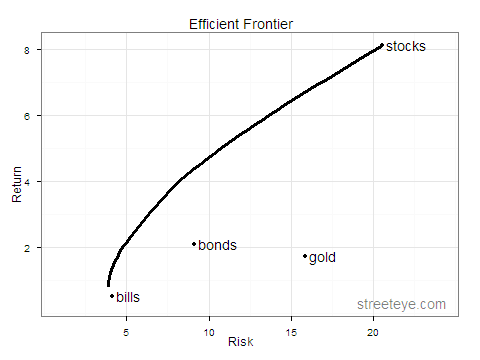
Efficient frontier plot:
1 2 3 4 5 6 7 8 9 10 11 12 13 14 15 16 17 18 19 20 21 22 23 24 |
require(ggplot2) # define colors dvblue = "#000099" dvred = "#e41a1c" dvgreen = "#4daf4a" dvpurple = "#984ea3" dvorange = "#ff7f00" dvyellow = "#ffff33" dvgray="#666666" apoints=data.frame(realsdspct) apoints$realreturns = realreturnspct ggplot(data=efrontier, aes(x=Risk, y=Return)) + opts(title="Efficient Frontier") + theme_bw() + geom_line(size=1.4) + geom_point(aes(x=apoints$realsdspct, y=apoints$realreturns)) + scale_x_continuous(limits=c(1,24)) + annotate("text", apoints[1,1], apoints[1,2],label=" stocks", hjust=) + annotate("text", apoints[2,1], apoints[2,2],label=" bills", hjust=) + annotate("text", apoints[3,1], apoints[3,2],label=" bonds", hjust=) + annotate("text", apoints[4,1], apoints[4,2],label=" gold", hjust=) + annotate("text", 19,0.3,label="streeteye.com", hjust=, alpha=0.5) |
You should see something like this:

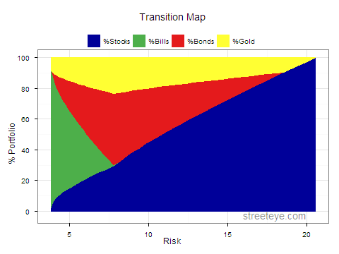
Transition map plot:
1 2 3 4 5 6 7 8 9 10 11 12 13 14 |
> keep=c("Risk", "%Stocks","%Bills","%Bonds","%Gold") > efrontier.tmp = efrontier[keep] > efrontier.m = melt(efrontier.tmp, id ='Risk') > > ggplot(data=efrontier.m, aes(x=Risk, y=value, colour=variable, fill=variable)) + + theme_bw() + + opts(title="Transition Map", legend.position="top", legend.direction="horizontal") + + ylab('% Portfolio') + + geom_area() + + scale_colour_manual("", breaks=c("%Stocks", "%Bills", "%Bonds","%Gold"), values = c(dvblue,dvgreen,dvred,dvyellow), labels=c('%Stocks', '%Bills','%Bonds','%Gold')) + + scale_fill_manual("", breaks=c("%Stocks", "%Bills", "%Bonds","%Gold"), values = c(dvblue,dvgreen,dvred,dvyellow), labels=c('%Stocks', '%Bills','%Bonds','%Gold')) + + annotate("text", 16,-2.5,label="streeteye.com", hjust=, alpha=0.5) > > |

That’s it…If you made it this far, congratulations! A few more R links to frustrate you are below. Now go forth, and enjoy beating your head against the wall!
