‘Cat Food’ revisited: testing dynamic spending rules - Part 1
How much can you safely spend out of a portfolio in retirement? Spend conservatively and you may be unnecessarily curbing the lifestyle and aspirations of you and your loved ones. Overspend and risk a shortfall and painful adjustment - in the extreme, the (hopefully apocryphal) “cat food” diet. A traditional rule of thumb is a fixed 4% per year of your starting portfolio, adjusted each year for inflation. A previous post discussed why this rule may not be safe:
- Low bond yields _ 1.8% for 10-year Treasurys and negative TIPS out to 10 years _ mean historical bond returns are mathematically unobtainable.1
- 2.2% real returns since 2000 on a 60/40 blended portfolio suggest that long-run return expectations need to be revisited. Low long-term interest rates are a forecast of low future returns, ie low growth and inflation expectations. To the extent equity risk premiums haven’t widened, they forecast lower than normal equity returns.
- Taxes and investment expenses must be included. Work supporting 4% tends to ignore them.
- US demographics are not very positive for growth, inflation, tax rates, and hence, real after-tax investment returns (which is reflected in the US fiscal position). The US dependency ratio is forecast to rise by 15 points over the next 20 years.
If the 4% rule hasn’t been decisively breached, forward-looking indicators are a bit worrisome. Could a more flexible rule not only be safer, but in favorable circumstances allow a higher level of spending? In this 3-part post, we test dynamic rules that vary withdrawal rates based on age and the size of the portfolio, and vary the composition of the portfolio over time.
Dynamic rule 1: Vary spending by age.
The first rule we’ll test is to spend a percentage of the actual portfolio each year (not a fixed percentage of the initial portfolio) and vary the percentage by age.
Suppose you are a 65 year old male. You have a life expectancy of 17.19 years per US government actuarial tables. It would make sense to vary spending as a percentage of your assets inversely with your life expectancy. As a base case you could spend 1/17.19=5.82% of your portfolio this year. Next year your life expectancy would be 16.48% You would spend 1/16.48=6.07%. This is higher than 4% for life expectancy < 25 years, but it’s an arbitrary base case _ just a starting point to test a rule based on the size of the portfolio and life expectancy.
Let’s apply this rule to a 60/40 stock/bond portfolio for someone who retired in 1928 to and see what spending it would have supported.
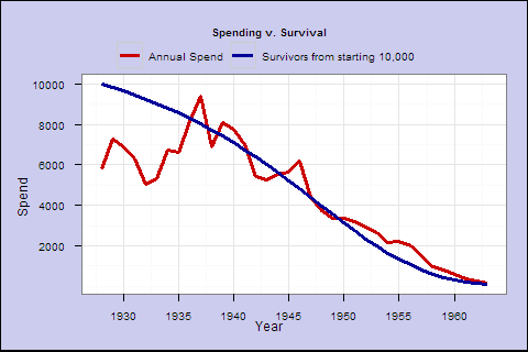
Figure 1. Inflation-adjusted spending for a 65-year-old single male who retires in 1928, with dynamic spending rule of 1/life_expectancy (spending factor=1) v. survival rate
This retiree would have experienced volatility, but he would really have started to go broke after around 1947, aged 85, shortly after his original life expectancy at retirement. From the blue survival line (from current life expectancy tables), over 40% would still have been alive for that drop. If he lived to be 100 after 35 years in 1963, he would have been penniless.
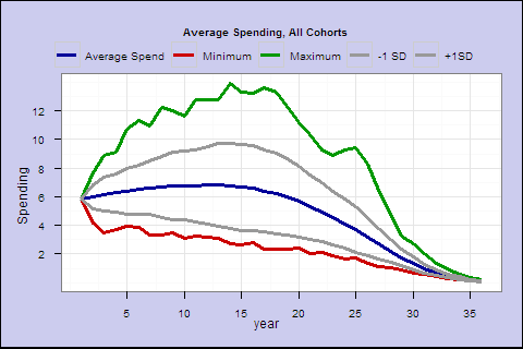
Is this rule too spendthrift, or was 1928 a particularly bad year to start retirement? Let’s try the same rule in all available 35-year retirement cohorts 1928-1977, and plot their average spending.
The middle blue line is the average income by retirement year. The green and red are the best and worst cases. The middle 2 lines represent the +/- 1 standard deviation confidence interval.
Even in the best case, you eventually go broke. Your life expectancy is 17.2 years at retirement, and on average your spending goes below the starting amount around year 19. This spending rule may not conservative enough.
Let’s call s spending factor, and try different spending rates s/life_expectancy. We can run spending factors between 0.05 and 1.2: Figure 3. Big chart panel (opens in new window). As we move toward the top of the page, we see safer profiles, and even the worst case scenarios start to seem fairly acceptable.
This exercise demonstrates the tradeoff between spending, and the risk of the average or worst-case income path exhibiting a major shortfall from the starting income.
To better visualize this big panel, we can estimate ‘lifetime spend expectancy’ and shortfall probability for each spending factor.
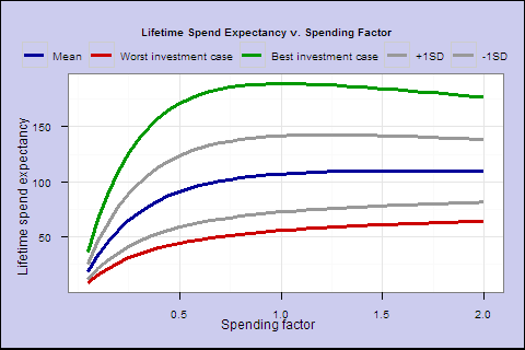
In Figure 4, for each year, we multiply the spending outcome by the probability of a cohort retiree surviving to that year, and sum up the years, to get the lifetime spend expectancy for a given spending factor. This summarizes each line in the Figure 3 panel as a single point, the expected lifetime spending as a percentage of starting portfolio.
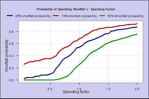
In Figure 5, for each s, we calculate the percentage of retirees in all cohorts who survived to a year where the spending falls to 25% below the initial spending.
These last 2 charts illustrate that as you increase the spending factor past 0.6, increasing lifetime spend expectancy flattens out, and the probability of 25% shortfall accelerates sharply.
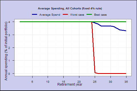
Finally, how does the fixed 4% rule compare? For a 65-year-old with a 60/40 portfolio, the 4% rule yields 70.4 expected lifetime spending with a 2% lifetime shortfall probability.
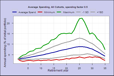
By comparison, a 0.5 spending factor, which starts at about 3% spending, yields expected spending of 91.2 with a 9.7% probability of a 25% drop from the initial spend amount, and a worst case drop of 37% (for 1973 retirees _ they eventually recovered).
But you do start at a lower rate, and spending is variable.
In the next post, we’ll test additional rules, to vary the composition of the portfolio by age, and to try smooth spending.
1The objection has been made that today’s rates can go lower and bond returns can be higher in the short run. True, but a 10-year bond bought at a yield of 1.8% will return, best case, 1.8% nominal over its lifetime (less in the event of default). If the yield goes to zero this year, it will return 18% this year, and zero over the rest of its lifetime. It’s called “fixed” income for a reason. When interest rates are below inflation, thinking bonds can be a real total return instrument in the base case is setting up for disappointment. It hasn’t been true historically, and it’s not what the market is pricing in. Bonds still have an important role as a liquidity and deflation hedge.
1 2 3 4 5 6 7 8 9 10 11 12 13 14 15 16 17 18 19 20 21 22 23 24 25 26 27 28 29 30 31 32 33 34 35 36 37 38 39 40 41 42 43 44 45 46 47 48 49 50 51 52 53 54 55 56 57 58 59 60 61 62 63 64 65 66 67 68 69 70 71 72 73 74 75 76 77 78 79 80 81 82 83 84 85 86 87 88 89 90 91 92 93 94 95 96 97 98 99 100 101 102 103 104 105 106 107 108 109 110 111 112 113 114 115 116 117 118 119 120 121 122 123 124 125 126 127 128 129 130 131 132 133 134 135 136 137 138 139 140 141 142 143 144 145 146 147 148 149 150 151 152 153 154 155 156 157 158 159 160 161 162 163 164 165 166 167 168 169 170 171 172 173 174 175 176 177 178 179 180 181 182 183 184 185 186 187 188 189 190 191 192 193 194 195 196 197 198 199 200 201 202 203 204 205 206 207 208 209 210 211 212 213 214 215 216 217 218 219 220 221 222 223 224 225 226 227 228 229 230 231 232 233 234 235 236 237 238 239 240 241 242 243 244 245 246 247 248 249 250 251 252 253 254 255 256 257 258 259 260 261 262 263 264 265 266 267 268 269 270 271 272 273 274 275 276 277 278 279 280 281 282 283 284 285 286 287 288 289 290 291 292 293 294 295 296 297 298 299 300 301 302 303 304 305 306 307 308 309 310 311 312 313 314 315 316 317 318 319 320 321 322 323 324 325 326 327 328 329 |
ageframe <- function (lifetable, age, maxage) { start = age+1 end=maxage+1 keep <- c("Age","Mmort","Mlives","MLE") retframe = lifetable[start:end,keep] retframe$survivepct=retframe$Mlives/retframe[1,"Mlives"] return(retframe) } cohortframe <- function (ageframe, portframe, startyear) { retframe <-ageframe retireyears=nrow(ageframe) endyear = startyear+retireyears-1 retframe$portreturn = portframe[startyear:endyear,"portreturn"] retframe$year = portframe[startyear:endyear,"Year"] return(retframe) } calcspending <- function(cohortframe, spendingfactor) { retframe <- cohortframe retframe$spend= retframe$startportval= retframe$endportval= portval=100 for (index in 1: nrow(retframe)) { myrow = retframe[index,] myrow["startportval"]=portval spendrate = spendingfactor/myrow["MLE"] spend = spendrate * portval myrow["spend"]=spend portval = portval - spend portval = portval * (1 + myrow["portreturn"]) myrow["endportval"]=portval retframe[index,]=myrow } return(retframe) } calcspendingfixed <- function(cohortframe, spendingfactor) { retframe <- cohortframe retframe$spend= retframe$startportval= retframe$endportval= portval=100 for (index in 1: nrow(retframe)) { myrow = retframe[index,] myrow["startportval"]=portval if ( portval > 4) { spend = 4 } else { spend <- portval } myrow["spend"] <- spend portval = portval - spend portval = portval * (1 + myrow["portreturn"]) myrow["endportval"]=portval retframe[index,]=myrow } return(retframe) } testspendingfactor <- function(realreturns, spendingfactor, minage, maxage) { tempageframe <- ageframe(lifetable, minage, maxage) ntrials <- nrow(realreturns)-nrow(tempageframe) +1 nyears <- maxage-minage+1 trials <- data.frame(1:nyears) colnames(trials) = "age" for (index in 1:ntrials) { tempframe1 = cohortframe(tempageframe,realreturns,index) tempframe2 = calcspending(tempframe1,spendingfactor) colname = paste("trial",index, sep="") trials[colname] <- tempframe2$spend } trials <- trials[2:ncol(trials)] return(trials) } testspendingfactorfixed <- function(realreturns, spendingfactor, minage, maxage) { tempageframe <- ageframe(lifetable, minage, maxage) ntrials <- nrow(realreturns)-nrow(tempageframe) +1 nyears <- maxage-minage+1 trials <- data.frame(1:nyears) colnames(trials) = "age" for (index in 1:ntrials) { tempframe1 = cohortframe(tempageframe,realreturns,index) tempframe2 = calcspendingfixed(tempframe1,spendingfactor) colname = paste("trial",index, sep="") trials[colname] <- tempframe2$spend } trials <- trials[2:ncol(trials)] return(trials) } calctrialssummary <- function(trials) { trialssummary <- data.frame(1:nrow(trials)) colnames(trialssummary) = "year" trialssummary$mean=apply(trials,1,mean) trialssummary$max=apply(trials,1,max) trialssummary$min=apply(trials,1,min) trialssummary$sd=apply(trials,1,sd) trialssummary$plus1sd=trialssummary$mean + trialssummary$sd trialssummary$minus1sd=trialssummary$mean - trialssummary$sd keep <- c("year", "mean","min","max","minus1sd","plus1sd") trialssummary <- trialssummary[,keep] return(trialssummary) } calcexpectedspending<- function(trials, survival) { trialssummary <- data.frame(1:nrow(trials)) colnames(trialssummary) = "year" trialssummary$survivepct=survival$survivepct trialssummary$mean=apply(trials,1,mean) trialssummary$expmean= trialssummary$mean * trialssummary$survivepct trialssummary$max=apply(trials,1,max) trialssummary$expmax= trialssummary$max * trialssummary$survivepct trialssummary$min=apply(trials,1,min) trialssummary$expmin= trialssummary$min * trialssummary$survivepct trialssummary$sd=apply(trials,1,sd) trialssummary$plus1sd=trialssummary$mean + trialssummary$sd trialssummary$expplus1sd= trialssummary$plus1sd * trialssummary$survivepct trialssummary$minus1sd=trialssummary$mean - trialssummary$sd trialssummary$expminus1sd= trialssummary$minus1sd * trialssummary$survivepct keep <- c("year", "expmean","expmin","expmax", "expplus1sd", "expminus1sd") trialssummary <- trialssummary[,keep] return(trialssummary) } chartsummary <- function(trialssummary, mytitle) { meltframe <- melt(trialssummary, id = 'year') ggplot(data=meltframe, aes(x=year, y=value, colour=variable)) + scale_x_continuous() + ylab("Annual spending (% of initial portfolio)") + xlab("Retirement year") + theme_bw() + geom_line(size=1.4) + opts(legend.position="top", legend.direction = 'horizontal', plot.background = theme_rect(colour = 'black', fill = '#CCCCEE', size = 1, linetype='solid')) + scale_colour_manual(mytitle, breaks = c('mean', 'min','max','minus1sd','plus1sd'), values = c("#000099", "#CC0000","#009900","#999999","#999999"), labels = c('Average Spend', 'Minimum', 'Maximum', '-1 SD', '+1SD')) } library(ggplot2) returns <- read.csv("~/Documents/returns.csv") # /assets/wp-content/uploads/2013/01/returns.csv lifetable <- read.csv("~/Documents/Lifetable.csv") # /assets/wp-content/uploads/2013/01/Lifetable.csv returns$realstocks=returns$Stocks-returns$CPI returns$realbonds=returns$Bonds-returns$CPI returns$realbills=returns$Bills-returns$CPI drops <- c("Stocks","Bonds","Bills","CPI") realreturns <- returns[,!(names(returns) %in% drops)] realreturns$portreturn = 0.6*realreturns$realstocks + 0.4 *realreturns$realbonds #Figure 1 tempageframe <- ageframe(lifetable, 65, 100) tempframe1 = cohortframe(tempageframe,realreturns,1) tempframe2 = calcspending(tempframe1,1) tempframe2$survival65 = tempframe2$survivepct * 10000 tempframe2$spend = tempframe2$spend * 1000 keep = c("year","spend","survival65" ) tempframe2 <- tempframe2[,keep] meltframe <- melt(tempframe2, id = 'year') ggplot(data=meltframe, aes(x=year, y=value, colour=variable)) + scale_x_continuous() + ylab("Spend") + xlab("Year") + theme_bw() + geom_line(size=1.4) + opts(legend.position="top", legend.direction = 'horizontal', plot.background = theme_rect(colour = 'black', fill = '#CCCCEE', size = 1, linetype='solid')) + scale_colour_manual("Annual spending, retirement age 65, 60/40 portfolio, spending factor 1, 1928 cohort", breaks = c('spend', 'survival65'), values = c("#CC0000", "#000099"), labels = c('Annual Spend', 'Survivors from starting 10,000')) #Figure 2 trials = testspendingfactor(realreturns, 1, 65, 100) trialssummary = calctrialssummary(trials) trialssummary$survival = ageframe65$survivepct*10000 keep <- c("year", "mean","min","max","minus1sd","plus1sd") trialssummary <- trialssummary[,keep] chartsummary(trialssummary, "Average Spending, All Cohorts") # Figure 3 facetframe = data.frame (year = integer(), variable=character(), value=double()) for (index in 1:24) { spendingfactor = index/20 trials = testspendingfactor(realreturns, spendingfactor, 65, 100) trialssummary = calctrialssummary(trials) trialssummary$spendingfactor = spendingfactor meltframe <- melt(trialssummary, id = c('year','spendingfactor')) facetframe <- merge(meltframe, facetframe, all=TRUE) } ggplot(data=facetframe, aes(x=year, y=value, colour=variable)) + scale_x_continuous() + ylab("Annual spending (% of initial portfolio)") + xlab("Retirement year") + theme_bw() + facet_wrap(~ spendingfactor, ncol = 4) + geom_line(size=1) + opts(legend.position="top", legend.direction = 'horizontal', plot.background = theme_rect(colour = 'black', fill = '#CCCCEE', size = 1, linetype='solid')) + scale_colour_manual("Average Spending, All Cohorts, Spending Factors 0.05 to 1.2", breaks = c('mean', 'min','max','minus1sd','plus1sd'), values = c("#000099", "#CC0000","#009900","#999999","#999999"), labels = c('Average Spend', 'Minimum', 'Maximum', '-1 SD', '+1SD')) ############################################################ ageframe65 = ageframe(lifetable,65,100) nsfactors = 40 sfactorsummary <- data.frame(1:nsfactors) colnames(sfactorsummary) = "year" sfactorsummary$sfactor <- sfactorsummary$expspend <- sfactorsummary$minspend <- sfactorsummary$maxspend <- sfactorsummary$plus1sd <- sfactorsummary$minus1sd <- sfactorsummary$sdspend <- sfactorsummary$shortfall <- for (index in 1:nsfactors) { spendingfactor = index/20 trials = testspendingfactor(realreturns, spendingfactor, 65, 100) trialssummary = calcexpectedspending(trials, ageframe65) sfactorsummary$sfactor[index] = spendingfactor sfactorsummary$expspend[index] = sum(trialssummary[,"expmean"]) sfactorsummary$minspend[index] = sum(trialssummary[,"expmin"]) sfactorsummary$maxspend[index] = sum(trialssummary[,"expmax"]) sfactorsummary$plus1sd[index] = sum(trialssummary[,"expplus1sd"]) sfactorsummary$minus1sd[index] = sum(trialssummary[,"expminus1sd"]) sfactorsummary$sdspend[index]=rowMeans(apply(trials, 2, sd)/trials[1,]) trialstmp=trials for (index2 in 1:ncol(trialstmp)) trialstmp[index2]=trialstmp[index2]/trialstmp[1,index2] trialstmp[trialstmp<0.75]=-1 trialstmp[trialstmp>]= trialstmp[trialstmp<]=1 for (index2 in 1:ncol(trialstmp)) trialstmp[index2]=trialstmp[index2] * ageframe65$survivepct sfactorsummary$shortfall[index]=mean(apply(trialstmp,2,max)) } chart1=sfactorsummary keep <- c("sfactor","expspend","minspend","maxspend","plus1sd","minus1sd") chart1 <- chart1[keep] meltframe <- melt(chart1, id = 'sfactor') ggplot(data=meltframe, aes(x=sfactor, y=value, colour=variable)) + scale_x_continuous() + ylab("Lifetime spend expectancy (% of initial portfolio)") + xlab("Spending factor") + theme_bw() + geom_line(size=1.4) + opts(legend.position="top", legend.direction = 'horizontal', plot.background = theme_rect(colour = 'black', fill = '#CCCCEE', size = 1, linetype='solid')) + scale_colour_manual("Lifetime Spend Expectancy v. Spending Factor", breaks = c('expspend', 'minspend','maxspend','plus1sd','minus1sd'), values = c("#000099", "#CC0000", "#009900","#999999","#999999"), labels = c('Mean', 'Worst investment outcome', 'Best investment outcome','+1SD','-1SD')) chart2=sfactorsummary keep <- c("sfactor","shortfall") chart2 <- chart2[keep] meltframe <- melt(chart2, id = 'sfactor') ggplot(data=meltframe, aes(x=sfactor, y=value, colour=variable)) + scale_x_continuous() + ylab("Shortfall probability") + xlab("Spending factor") + theme_bw() + geom_line(size=1.4) + opts(legend.position="top", legend.direction = 'horizontal', plot.background = theme_rect(colour = 'black', fill = '#CCCCEE', size = 1, linetype='solid')) + scale_colour_manual("Probability of 25% Spending Shortfall v. Spending Factor", breaks = c('shortfall'), values = c("#000099"), labels = c('Shortfall probability')) # fixed 4% rule trials = testspendingfactorfixed(realreturns, 1, 65, 100) trialssummary = calctrialssummary(trials) ageframe65 = ageframe(lifetable,65,100) trialssummary$survivepct=ageframe65$survivepct trialssummary$expmean = trialssummary$mean * trialssummary$survivepct sum(trialssummary$expmean) trials[trials<4]=-1 trials[trials>]= trials[trials<]=1 trials[,]=trials[,] * ageframe65$survivepct mean(apply(trials,2,max)) # 0.5 spending factor -> look up from sfactorsummary |
