Retirement plans that maximize certainty-equivalent spending (conclusion)
In part 1 and part 2, we developed a framework for evaluating and identifying a good plan for retirement spending and asset allocation.
- We discussed how a CRRA (constant relative risk aversion) utility function and the related concept of certainty-equivalent (CE) spending can discount a stream of future cash flows based on their risk and variability, and the retiree’s risk aversion.
- We solved a toy problem: how the retiree maximizes certainty-equivalent spending if he or she can invest at a guaranteed fixed risk-free real return rate.
- We generated CE-optimal spending schedules using that fixed risk-free real return rate for retirees with different levels of risk aversion (in this case, no investment risk, just longevity risk, trading off current income for future risk of outliving the portfolio)
- We moved from a fixed rate assumption to using historical US real returns on stocks and bonds. We generated a spending schedule that maximized CE spending based on historical real returns for a 50% equity portfolio.
- Using that spending schedule, we solved the other side of the problem, and generated an equity allocation that would have maximized CE spending for that spending schedule.
- We looked at that solution, and found it seemed pretty good.
So, where we left off, we had independently solved the spending schedule and then the equity allocation schedule. Of course, that does not mean that when you put those two solutions together, they are the best we can do. It just means the equity allocation is the best available given that spending schedule. So today, we’ll try to solve them simultaneously.
The framework in which we try to solve the retirement spending problem is:
_Maximize expected CE spending for a 25-year retirement…
Which is modeled as a function of a 2×25 matrix
• 25-years of retirement
• Spending % each year
• Equity % each year (the balance to be allocated to bonds)
_
And we find CE spending as:
_Starting with the 2×25 vector of portfolio allocations and spending %
-> generate cash flows using historical returns for each retirement cohort
-> compute CE spending using CRRA function and gamma
-> compute expected CE spending for each cohort based on life table
-> compute expected CE spending across all cohorts and across all survival scenarios
_
That gives us a value: the CE spending a random retiree at any year 1926-1987, with the given life table, and given risk aversion, could have expected from that 2×25 spending/allocation schedule.
Now, the problem is to maximize that value: find the 2×25 spending/allocation schedule that maximizes the CE spending function.
So we fire up our optimizer, using this function, gamma=4, and the starting solution we previously found solving the two schedules independently. We try a few different optimization methods. Some of them fail, but the Powell method comes up with a pretty good solution after about six hours on our PC. We use that as our starting solution and run the optimization again using several different methods, and with a very slight improvement it holds up as the best we can find.
| Age | Equity % | Spending % |
| 65 | 63.8% | 6.1% |
| 66 | 63.7% | 6.4% |
| 67 | 72.1% | 6.7% |
| 68 | 73.7% | 6.9% |
| 69 | 74.4% | 7.2% |
| 70 | 75.2% | 7.5% |
| 71 | 85.3% | 7.9% |
| 72 | 86.1% | 8.3% |
| 73 | 75.3% | 8.7% |
| 74 | 76.8% | 9.2% |
| 75 | 80.9% | 9.8% |
| 76 | 86.3% | 10.5% |
| 77 | 91.6% | 11.3% |
| 78 | 100.0% | 12.2% |
| 79 | 98.9% | 13.0% |
| 80 | 100.0% | 14.1% |
| 81 | 100.0% | 15.3% |
| 82 | 100.0% | 16.6% |
| 83 | 100.0% | 18.5% |
| 84 | 100.0% | 20.9% |
| 85 | 100.0% | 24.1% |
| 86 | 100.0% | 28.8% |
| 87 | 100.0% | 36.8% |
| 88 | 100.0% | 52.8% |
| 89 | 50.0% | 100.0% |
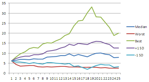
We see that our initial spending is higher (6.1% vs. 5.9% when we optimized spending and equity independently). We see that in our median case, spending is flatter. We see that the worst-case outcome is a bit worse. Nevertheless it seems credible that the tradeoff is preferable for a moderately risk averse retiree.
Actual spending using computed schedule, % of initial portfolio, 25-year retirement cohorts 1926-1987
It’s quite interesting that the equity % starts at 63.8% and rises throughout retirement. Conventional wisdom, as implemented in many target date funds would be to reduce the equity allocation as you get older, since you have less time to recover any shortfall from a major market decline. So that result bears investigation to see if there is an error, or if it’s inherent in the unconventional aspects of this approach.
Otherwise, this seems like an analytically sound approach that yields a good practical result.
Comments are invited.