Gold as Part of a Long-Run Asset Allocation (update)
You have to choose between trusting to the natural stability of gold and the natural stability of the honesty and intelligence of the members of the government. And, with due respect to these gentlemen, I advise you, as long as the capitalist system lasts, to vote for gold. - George Bernard Shaw
Here’s a quick update of a post I did a couple of years back on Gold as part of a long run asset allocation. Gold hasn’t fared too well since then. Is it still worth owning?
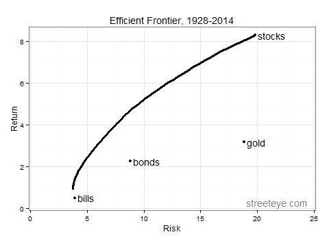
Let’s look at four asset classes from 1928-2014: US stocks (ie S&P), medium-term Treasurys (ie 10-year), T-bills, and gold. (Would love to do international developed, emerging, TIPS, real estate, but data doesn’t go back that far.)
Let’s adjust returns for inflation. Here’s are the historical mean annual real returns and standard deviations of annual returns.
| Real Return | Real Risk | |||
| Stocks | 8.3% | 19.8% | ||
| Bonds | 2.3% | 8.8% | ||
| Bills | 0.5% | 3.9% | Gold | 3.2% | 18.8% | </tr>
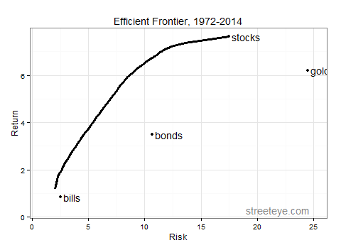
Let’s compute the efficient frontier. The left-most point is the minimum-volatility portfolio. The right-most point is the max-return portfolio, which is 100% stocks. We compute the minimum-volatility portfolio for return levels between those two, and plot the resulting efficient frontier.
 </p>
</p>
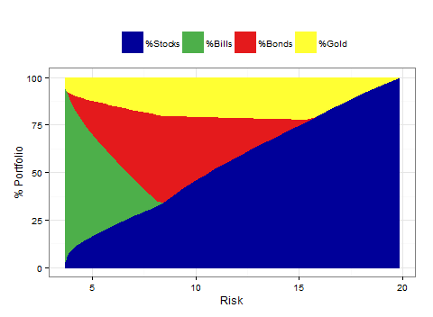
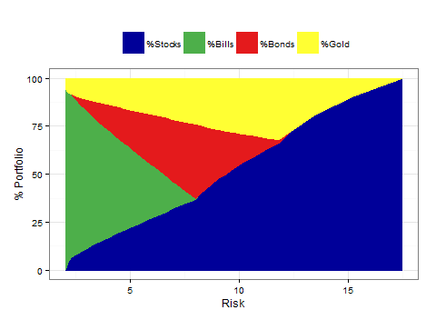
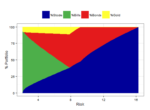
What is the composition of the portfolio at each point on the efficient frontier? We plot a transition map showing that as you start from the minimum-volatility portfolio with about 1% real return and 2% volatility, composed of mostly T-bills, with some stocks and gold, and move toward the maximum-return portfolio, you add more and more stocks, but always include some gold.
Transition map, 1926-2014
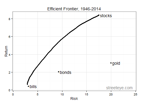
Let’s try a few different eras.
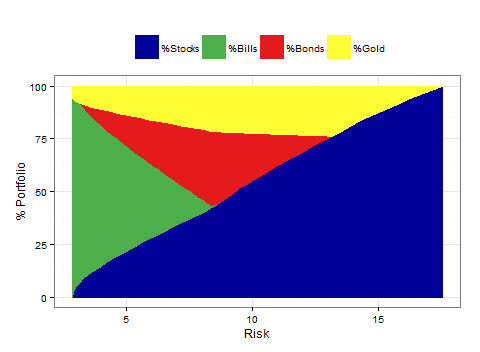
**1946-2014, Post-war, since Bretton Woods:
**
1972-2010, Post-war, post-gold standard (had to adjust the scale a little to get that gold data point on there):
1982-2014, era of disinflation:
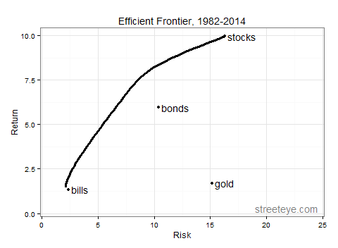
What should one conclude? In most regimes gold was worth owning in the portfolio that gives the most return at a given risk level. The exception was the era of globalization and disinflation, where we had high returns from stocks coupled with disinflation. If you expect that to be the case, as it has been the last 30 years, gold doesn’t improve the longer time-frame, more risky portfolios, like a 70-30 portfolio. But over the varied regimes of the last 87 years, it was a hedge worth having.
I say this as one who believes the gold bugs are useless, except for a chuckle. But central banks really want moderate inflation to solve the consumer debt/balance sheet problem. Deflation is anathema to them when everyone is up to their eyeballs in debt.
The question of our time is whether QE/easing -> inflated asset values -> more debt -> consumer goods/services inflation -> solves debt and overinflated asset problem.
Or QE/easing -> more debt -> deflation/no inflation -> even more precarious balance sheets -> financial crises and economic chaos.
Either way, a little gold is a good hedge in a number of scenarios.
(See the whole Bernanke/Summers/Piketty secular stagnation/robots debate, which I discussed a bit here.)
R code and data:
# install.packages('quantmod') # require(quantmod) # install.packages('lpSolve') require(lpSolve) # install.packages('quadprog') require(quadprog) # install.packages('ggplot2') require(ggplot2) require(reshape) # define functions ################################################################# # use linear programming to find maximum return portfolio (100% highest return asset) ################################################################# runlp <- function ( returns ) { # find maximum return portfolio (rightmost point of efficient frontier) # will be 100% of highest return asset # maximize # w1 * stocks return +w2 *bills +w3*bonds + w4 * gold # subject to 0 <= w <= 1 for each w # will pick highest return asset with w=1 # skipping >0 constraint, no negative return assets, so not binding opt.objective <- apply(returns, 2, mean) # should use length(objective) to populate matrix nAssets <- length(returns) ones = rep (1, nAssets) zeros = rep (, nAssets) # constrain sum of weights to 1 constraintlist = ones operatorlist = c("=") rhslist = c(1) # constrain each weight >= 0 for(i in 1:nAssets) { newconstraint = zeros newconstraint[i]=1 constraintlist = c(constraintlist, newconstraint) operatorlist = c(operatorlist, ">=") rhslist = c(rhslist, ) } # Example # opt.constraints <- matrix (c(1, 1, 1, 1, # constrain sum of weights to 1 # 1, 0, 0, 0, # constrain w1 <= 1 # 0, 1, 0, 0, # constrain w2 <= 1 # 0, 0, 1, 0, # constrain w3 <= 1 # 0, 0, 0, 1) # constrain w4 <= 1 # , nrow=5, byrow=TRUE) opt.constraints <- matrix (constraintlist, nrow=nAssets+1, byrow=TRUE) opt.operator <- operatorlist opt.rhs <- rhslist opt.dir="max" tmpsolution = lp (direction = opt.dir, opt.objective, opt.constraints, opt.operator, opt.rhs) sol= c() # portfolio weights for max return portfolio sol$wts=tmpsolution$solution # return for max return portfolio sol$ret=tmpsolution$objval # compute return covariance matrix to determine volatility of this portfolio sol$covmatrix = cov(returns, use = 'complete.obs', method = 'pearson') # multiply weights x covariances x weights, gives variance sol$var = sol$wts %*% sol$covmatrix %*% sol$wts # square root gives standard deviation (volatility) sol$vol = sqrt(sol$var) return (sol) } runqp <- function ( returns, hurdle= ) { ################################################################# # find minimum volatility portfolio ################################################################# # minimize variance: w %*% covmatrix %*% t(w) # subject to sum of ws = 1 # subject to each w >= 0 # subject to each return >= hurdle # solution.minvol <- solve.QP(covmatrix, zeros, t(opt.constraints), opt.rhs, meq = opt.meq) # first 2 parameters covmatrix, zeros define function to be minimized # if zeros is all 0s, the function minimized ends up equal to port variance / 2 # opt.constraints is the left hand side of the constraints, ie the cs in # c1 w1 + c2 w2 ... + cn wn = K # opt.rhs is the Ks in the above equation # meq means the first meq rows are 'equals' constraints, remainder are >= constraints # if you want to do a <= constraint, multiply by -1 to make it a >= constraint # does not appear to accept 0 RHS, so we make it a tiny number> 0 # compute expected returns meanreturns <- apply(returns, 2, mean) # compute covariance matrix covmatrix = cov(returns, use = 'complete.obs', method = 'pearson') nAssets <- length(returns) nObs <- length(returns$stocks) ones = rep (1, nAssets) zeros = rep (, nAssets) # constrain sum of weights to 1 constraintlist = ones rhslist = c(1) # constrain each weight >= 0 for(i in 1:nAssets) { newconstraint = zeros newconstraint[i]=1 constraintlist = c(constraintlist, newconstraint) rhslist = c(rhslist, ) } # constrain return >= hurdle constraintlist = c(constraintlist, meanreturns) rhslist = c(rhslist, hurdle) # example # opt.constraints <- matrix (c(1, 1, 1, 1, # sum of weights =1 # 1, 0, 0, 0, # w1 >= 0 # 0, 1, 0, 0, # w2 >= 0 # 0, 0, 1, 0, # w3 >= 0 # 0, 0, 0, 1) # w4 >= 0 # , nrow=5, byrow=TRUE) # opt.rhs <- matrix(c(1, 0.000001, 0.000001, 0.000001, 0.000001)) # opt.constraints = rbind(opt.constraints, meanreturns) # opt.rhs=rbind(opt.rhs, hurdle) opt.constraints <- matrix (constraintlist, nrow=nAssets+2, byrow=TRUE) opt.rhs <- opt.rhs <- matrix(rhslist) opt.meq <- 1 # first constraint is '=', rest are '>=' zeros <- array(, dim = c(nAssets,1)) tmpsolution <- solve.QP(covmatrix, zeros, t(opt.constraints), opt.rhs, meq = opt.meq) sol= c() sol$wts = tmpsolution$solution sol$var = tmpsolution$value *2 sol$ret = meanreturns %*% sol$wts sol$vol = sqrt(sol$var) return(sol) } loopqp <- function (minvol, maxret, numtrials) { ################################################################# # loop and run a minimum volatility optimization for each return level from 2-49 ################################################################# # put minreturn portfolio in return series for min return, index =1 out.ret=c(minvol$ret) out.vol=c(minvol$vol) out.stocks=c(minvol$wts[1]) out.bills=c(minvol$wts[2]) out.bonds=c(minvol$wts[3]) out.gold=c(minvol$wts[4]) lowreturn <- minvol$ret highreturn <- maxret$ret minreturns <- seq(lowreturn, highreturn, length.out=numtrials) for(i in 2:(length(minreturns) - 1)) { tmpsol <- runqp(freal,minreturns[i]) tmp.wts = tmpsol$wts tmp.var = tmpsol$var out.ret[i] = realreturns %*% tmp.wts out.vol[i] = sqrt(tmp.var) out.stocks[i]=tmp.wts[1] out.bills[i]=tmp.wts[2] out.bonds[i]=tmp.wts[3] out.gold[i]=tmp.wts[4] } # put maxreturn portfolio in return series for max return out.ret[numtrials]=c(maxret$ret) out.vol[numtrials]=c(maxret$vol) out.stocks[numtrials]=c(maxret$wts[1]) out.bills[numtrials]=c(maxret$wts[2]) out.bonds[numtrials]=c(maxret$wts[3]) out.gold[numtrials]=c(maxret$wts[4]) efrontier=data.frame(out.ret*100) efrontier$vol=out.vol*100 efrontier$stocks=out.stocks*100 efrontier$bills=out.bills*100 efrontier$bonds=out.bonds*100 efrontier$gold=out.gold*100 names(efrontier) = c("Return", "Risk", "%Stocks", "%Bills", "%Bonds", "%Gold") return(efrontier) } ############################################################ # charts ############################################################ plot_efrontier <- function (efrontier, returns, sds, apoints, title) { ggplot(data=efrontier, aes(x=Risk, y=Return)) + theme_bw() + geom_line(size=1.4) + geom_point(data=apoints, aes(x=Risk, y=Return)) + scale_x_continuous(limits=c(1,24)) + ggtitle(title) + annotate("text", apoints[1,1], apoints[1,2],label=" stocks", hjust=) + annotate("text", apoints[2,1], apoints[2,2],label=" bills", hjust=) + annotate("text", apoints[3,1], apoints[3,2],label=" bonds", hjust=) + annotate("text", apoints[4,1], apoints[4,2],label=" gold", hjust=) + annotate("text", 19,0.3,label="streeteye.com", hjust=, alpha=0.5) } plot_transitionmap <- function (efrontier, returns, sds) { # define colors dvblue = "#000099" dvred = "#e41a1c" dvgreen = "#4daf4a" dvpurple = "#984ea3" dvorange = "#ff7f00" dvyellow = "#ffff33" dvgray="#666666" efrontier.m = melt(efrontier, id ='Risk') ggplot(data=efrontier.m, aes(x=Risk, y=value, colour=variable, fill=variable)) + theme_bw() + theme(legend.position="top", legend.direction="horizontal") + ylab('% Portfolio') + geom_area() + scale_colour_manual("", breaks=c("%Stocks", "%Bills", "%Bonds","%Gold"), values = c(dvblue,dvgreen,dvred,dvyellow), labels=c('%Stocks', '%Bills','%Bonds','%Gold')) + scale_fill_manual("", breaks=c("%Stocks", "%Bills", "%Bonds","%Gold"), values = c(dvblue,dvgreen,dvred,dvyellow), labels=c('%Stocks', '%Bills','%Bonds','%Gold')) # annotate("text", 16,-2.5,label="streeteye.com", hjust=0, alpha=0.5) } ################################################################# # Create some data ################################################################# # sources: # http://pages.stern.nyu.edu/~adamodar/New_Home_Page/datafile/histretSP.html # http://www.onlygold.com/Info/Historical-Gold-Prices.asp # http://www.spdrgoldshares.com/usa/historical-data/ ################################################################# # not used in abbreviated example, but useful for reporting startYear = 1928 endYear = 2014 YEARS =startYear:endYear # nominal returns # nominal returns SP500 = c(0.4381,-0.083,-0.2512,-0.4384,-0.0864,0.4998,-0.0119,0.4674,0.3194,-0.3534,0.2928,-0.011, -0.1067,-0.1277,0.1917,0.2506,0.1903,0.3582,-0.0843,0.052,0.057,0.183,0.3081,0.2368,0.1815, -0.0121,0.5256,0.326,0.0744,-0.1046,0.4372,0.1206,0.0034,0.2664,-0.0881,0.2261,0.1642,0.124, -0.0997,0.238,0.1081,-0.0824,0.0356,0.1422,0.1876,-0.1431,-0.259,0.37,0.2383,-0.0698,0.0651, 0.1852,0.3174,-0.047,0.2042,0.2234,0.0615,0.3124,0.1849,0.0581,0.1654,0.3148,-0.0306,0.3023, 0.0749,0.0997,0.0133,0.372,0.2268,0.331,0.2834,0.2089,-0.0903,-0.1185,-0.2197,0.2836,0.1074, 0.0483,0.1561,0.0548,-0.3655,0.2594,0.1482,0.021,0.1589,0.3215,0.1348) BILLS = c(0.0308,0.0316,0.0455,0.0231,0.0107,0.0096,0.0032,0.0018,0.0017,0.003,0.0008,0.0004, 0.0003,0.0008,0.0034,0.0038,0.0038,0.0038,0.0038,0.0057,0.0102,0.011,0.0117,0.0148, 0.0167,0.0189,0.0096,0.0166,0.0256,0.0323,0.0178,0.0326,0.0305,0.0227,0.0278,0.0311, 0.0351,0.039,0.0484,0.0433,0.0526,0.0656,0.0669,0.0454,0.0395,0.0673,0.0778,0.0599, 0.0497,0.0513,0.0693,0.0994,0.1122,0.143,0.1101,0.0845,0.0961,0.0749,0.0604,0.0572, 0.0645,0.0811,0.0755,0.0561,0.0341,0.0298,0.0399,0.0552,0.0502,0.0505,0.0473,0.0451, 0.0576,0.0367,0.0166,0.0103,0.0123,0.0301,0.0468,0.0464,0.0159,0.0014,0.0013,0.0003, 0.0005,0.0007,0.0005) BONDS=c(0.0084,0.042,0.0454,-0.0256,0.0879,0.0186,0.0796,0.0447,0.0502,0.0138,0.0421,0.0441, 0.054,-0.0202,0.0229,0.0249,0.0258,0.038,0.0313,0.0092,0.0195,0.0466,0.0043,-0.003, 0.0227,0.0414,0.0329,-0.0134,-0.0226,0.068,-0.021,-0.0265,0.1164,0.0206,0.0569,0.0168, 0.0373,0.0072,0.0291,-0.0158,0.0327,-0.0501,0.1675,0.0979,0.0282,0.0366,0.0199,0.0361, 0.1598,0.0129,-0.0078,0.0067,-0.0299,0.082,0.3281,0.032,0.1373,0.2571,0.2428,-0.0496, 0.0822,0.1769,0.0624,0.15,0.0936,0.1421,-0.0804,0.2348,0.0143,0.0994,0.1492,-0.0825, 0.1666,0.0557,0.1512,0.0038,0.0449,0.0287,0.0196,0.1021,0.201,-0.1112,0.0846,0.1604, 0.0297,-0.091,0.1075) CPI=c(-0.0115607,0.005848,-0.0639535,-0.0931677,-0.1027397,0.0076336,0.0151515,0.0298507, 0.0144928,0.0285714,-0.0277778,,0.0071429,0.0992908,0.0903226,0.0295858,0.0229885, 0.0224719,0.1813187,0.0883721,0.0299145,-0.0207469,0.059322,0.06,0.0075472,0.0074906, -0.0074349,0.0037453,0.0298507,0.0289855,0.0176056,0.017301,0.0136054,0.0067114,0.0133333, 0.0164474,0.0097087,0.0192308,0.0345912,0.0303951,0.0471976,0.0619718,0.0557029,0.0326633, 0.0340633,0.0870588,0.1233766,0.0693642,0.0486486,0.0670103,0.0901771,0.1329394,0.125163, 0.0892236,0.0382979,0.0379098,0.0394867,0.0379867,0.010979,0.0443439,0.0441941,0.046473, 0.0610626,0.0306428,0.0290065,0.0274841,0.026749,0.0253841,0.0332248,0.017024,0.016119, 0.0268456,0.0338681,0.0155172,0.0237691,0.0187949,0.0325556,0.0341566,0.0254065,0.0408127, 0.0009141,0.0272133,0.0149572,0.03,0.017,0.015,0.008) GOLD = c(,,,,,0.563618771,0.082920792, ,,,,,-0.014285714,0.028985507,, 0.028169014,-0.006849315,0.027586207,0.026845638,0.124183007,-0.023255814,-0.035714286, -0.00617284,-0.00621118,-0.0325,-0.082687339,-0.007042254,-0.002836879,0.001422475, 0.001420455,,,0.035460993,-0.02739726,-0.004225352,-0.002828854, 0.002836879,0.004243281,-0.002816901,0.002824859,0.225352113,-0.057471264,-0.051219512, 0.146529563,0.431390135,0.667919799,0.725864012,-0.242041683,-0.03962955,0.204305898, 0.291744258,1.205670351,0.296078431,-0.327618087,0.1175,-0.149888143,-0.189473684, 0.061688312,0.195412844,0.244563827,-0.156937307,-0.022308911,-0.036907731,-0.085577421, -0.057057907,0.176426426,-0.021697511,0.009784736,-0.046511628,-0.222086721,0.005748128, 0.005368895,-0.060637382,0.014120668,0.23960217,0.217359592,0.04397843,0.17768595, 0.231968811,0.319224684,0.043178411,0.250359299,0.292413793,0.089292067,0.082625735, -0.273303167,0.00124533 ) # truncate here, e.g. # 1928 - 2014 - 87 years # 1946 - 2014 - 69 years #SP500=SP500[19:87] #BILLS=BILLS[19:87] #BONDS=BONDS[19:87] #GOLD=GOLD[19:87] #CPI=CPI[19:87] # 1972 - 2014 - 43 years # SP500=SP500[45:87] # BILLS=BILLS[45:87] # BONDS=BONDS[45:87] # GOLD=GOLD[45:87] # CPI=CPI[45:87] # 1982 - 2014 - 33 years SP500=SP500[55:87] BILLS=BILLS[55:87] BONDS=BONDS[55:87] GOLD=GOLD[55:87] CPI=CPI[55:87] # put into a data frame fnominal=data.frame(stocks=SP500, bills=BILLS, bonds=BONDS, gold=GOLD, CPI=CPI) freal=data.frame(stocks=(1+SP500)/(1+CPI)-1, bills=(1+BILLS)/(1+CPI)-1, bonds=(1+BONDS)/(1+CPI)-1, gold=(1+GOLD)/(1+CPI)-1) #freal=data.frame(stocks=SP500-CPI, bills=BILLS-CPI, bonds=BONDS-CPI, gold=GOLD-CPI) # compute real return means realreturns = apply(freal, 2, mean) realreturnspct = realreturns*100 # print them realreturnspct # compute real return volatility (standard deviation of real returns) realsds = apply(freal, 2, sd) realsdspct = realsds*100 # print them realsdspct maxret <- runlp(freal) minvol <- runqp(freal,) # generate a sequence of 50 evenly spaced returns between min var return and max return efrontier = loopqp(minvol, maxret, 50) apoints <- data.frame(realsdspct) apoints$returns <- realreturnspct names(apoints) = c("Risk", "Return") plot_efrontier(efrontier, realreturnspct, realsdspct, apoints, "Efficient Frontier, 1946-2014") keep=c("Risk", "%Stocks","%Bills","%Bonds","%Gold") plot_transitionmap(efrontier[keep], realreturnspct, realsdspct) |